Filter Events by Year
MSc. Personalised Medicine, Computational Genomics Module, University College London: Ensembl Variation Data and the VEP
Course Details
- Lead Trainer
- Aleena Mushtaq
- Event Date
- 2024-01-30
- Location
- London
- Description
- Work with the Ensembl Outreach team to get hands-on experience accessing and analysing variation data with the Ensembl genome browser.
- Survey
- MSc. Personalised Medicine, Computational Genomics Module, University College London: Ensembl Variation Data and the VEP Feedback Survey
Demos and exercises
Species and genome assemblies
Demo: Introduction to Ensembl
Ensembl
Homepage
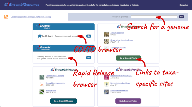
The front page of Ensembl is found at ensembl.org. It contains lots of information and links to help you navigate Ensembl:
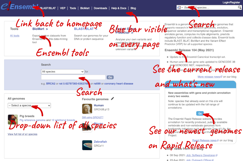
On the right-hand panel you can see the current release number and what has come out in this release. To access old releases, scroll to the bottom of the page and click on View in archive site in the right-hand corner.
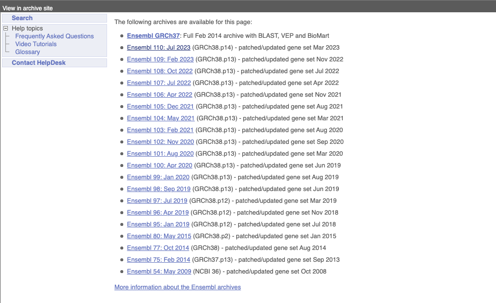
Click on the links to go to the archives. Alternatively, you can jump quickly to the correct release by adding e plus the release number in the URL. For example e98.ensembl.org jumps to Ensembl release 98.
Available species
Scroll back up to the top of the homepage. You can view all available species by clicking the View full list of all species link underneath the coloured search block.
You can search for your species of interest (either the common or scientific name) using the search bar at the top right-hand corner of the table. Click on the common name of your species of interest to go to the species information page. We’ll click on Human.
Species information
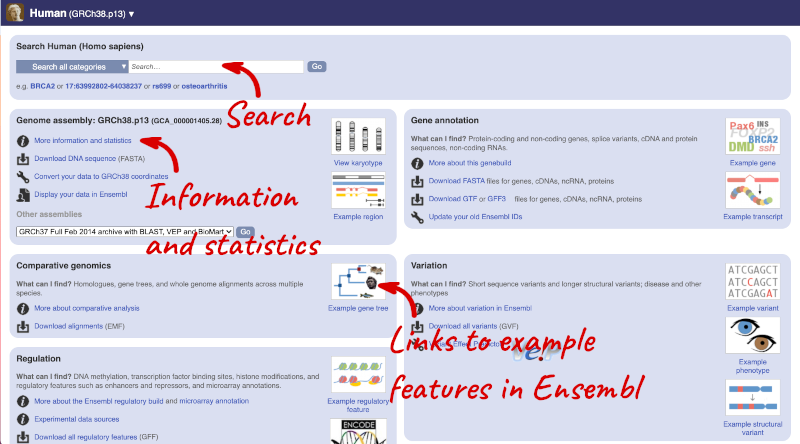
Here you can see links to example features and to download flatfiles. To find out more about the genome assembly and genebuild, click on More information and statistics under the Genome assembly section.
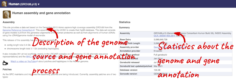
Here you’ll find a detailed description of how to the genome was produced and links to the original source. You will also see details of how the genes were annotated.
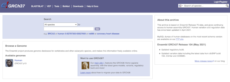
The current genome assembly for human is GRCh38. If you want to see the previous assembly, GRCh37, visit our dedicated site grch37.ensembl.org.
Ensembl Genomes
Homepage
Let’s take a look at the Ensembl Genomes homepage at ensemblgenomes.org.
Click on the different taxa to see their homepages. Each one has a different colour-coding, but they are all structured in a similar format to the Ensembl main site.
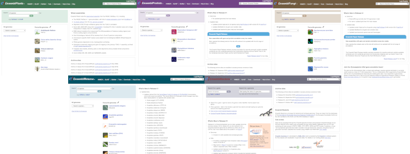
You can navigate most of the taxa in the same way as you would with Ensembl.
Ensembl Bacteria
Ensembl Bacteria has a large number of genomes and has a slightly different method to the other Ensembl sites. Let’s look at it in more detail.
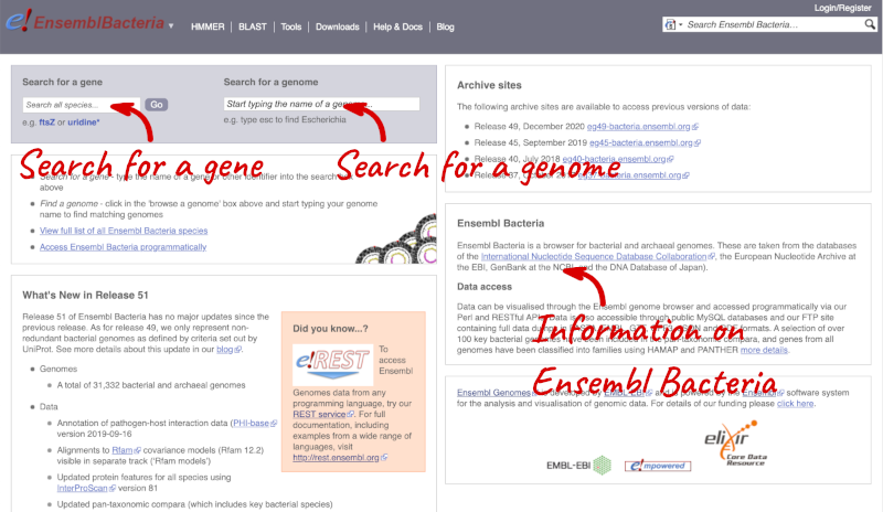
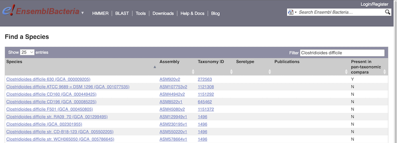
There’s no drop-down species list for bacteria as it would be hard to navigate with the number of species. You can click the View full list of all Ensembl Bacteria species link underneath the coloured search block. Search for your species of interest using the filter in the top right-hand corner of the table.
Alternatively, you can find a species by typing the species name into the Search for a genome search box at the top of the page. A drop-down list will appear with any species matching the name you entered.
For example, to find a sub-strain of Clostridioides difficile start typing in the species name. Due to the auto-complete, you’ll see useful results as soon as you get to Clostridio.
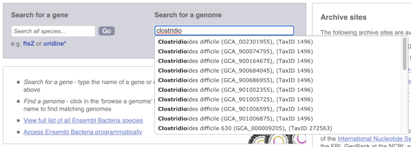
The drop down contains various strains of C. difficile. Let’s choose C. difficile 630. This will take us to another species information page, where we can explore various features.
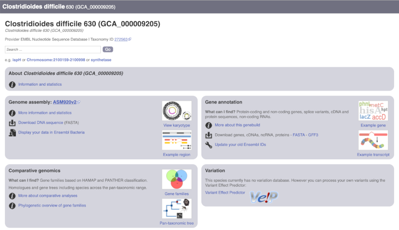
Unlike the Homo sapiens species information page, there is no prose description of the genome or gene annotation, as these pages were generated automatically.
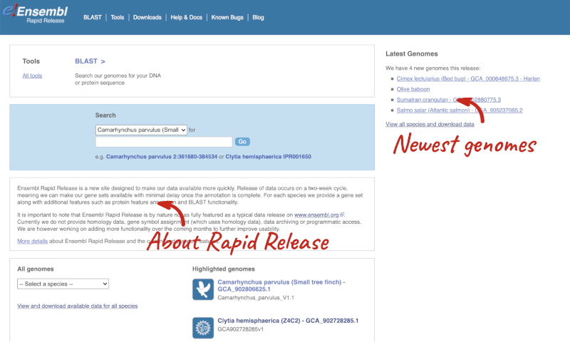
Ensembl Rapid Release
Our newest genomes, such as those coming from the Darwin Tree of Life, are available rapid.ensembl.org with limited annotation.
Panda species
Go to Ensembl and find the following information:
-
What is the name of the genome assembly for Panda?
-
How long is the Panda genome (in bp)? How many coding genes have been annotated?
-
Select Giant panda from the drop down species list, or click on View full list of all Ensembl species, then choose Giant panda from the list.
The assembly is ASM200744v2 or GCA_002007445.2. -
Click on More information and statistics. Statistics are shown in the tables on the left.
The length of the genome is 2,444,060,653 bp.
There are 20,857 coding genes.
Available zebrafish assemblies
What previous assemblies are available for zebrafish?
Click on Zebrafish on the front page of Ensembl to go to the species homepage. Under Other assemblies three previous assembly names and the releases you can find them in are listed.
Assembly GRCz10 is available in the archived release 80, Zv9 in 77 and Zv8 in 54.
Solanum genus
Go to Ensembl Plants and answer the following questions:
-
How many genomes of the genus Solanum are there in Ensembl Plants?
-
When was the current Solanum lycopersicum genome assembly last revised?
- On the homepage, click on View full list of all Ensembl Plants species underneath the coloured search block. Type Solanum into the filter box in the top left-hand corner of the table.
There are three Solanum genomes: Solanum lycopersicum (tomato), and Solanum tuberosum RH89-039-16 and Solanum tuberosum (both potato).
- Click on S. lycopersicum, then on More information and statistics.
The genome was revised in April 2018.
Mosquito species
-
Go to Ensembl Metazoa. How many genomes relating to the genus Anopheles are there in Ensembl Metazoa?
-
When was the current Anopheles gambiae genome assembly last revised?
- Go to metazoa.ensembl.org. Open the drop-down list or click on View full list of all Ensembl Metazoa species. In a latin binomial species name, the first word represents the genus. Type Anopheles into the filter box in the top left to find all genomes with this word in the binomial.
There are 22 Anopheles genomes (some species are represented by more than one genome).
- Click on Anopheles gambiae (African malaria mosquito, PEST), and then on More information and statistics.
The assembly hosted is AgamP4 (INSDC Assembly GCA_000005575.1) which was revised in Feb 2006.
Finding a genome in Ensembl Bacteria
Mycobacterium tuberculosis H37Ra str. ATCC25177 is a clinical strain.
Go to Ensembl Bacteria and find the species M. tuberculosis H37Ra str. ATCC25177. How many coding genes does it have?
In the Ensesmbl Bacteria homepage, start to type H37Ra into the Search for a genome search box (you can find this in the coloured block at the top of the homepage). It will auto-complete, allowing you to select M. tuberculosis H37Ra str. ATCC25177 from the drop-down list. Click on More information and statistics.
M. tuberculosis H37Ra str. ATCC25177 has 4,080 coding and 47 non-coding genes.
Exploring genomic regions
Start at the Ensembl front page, ensembl.org. You can search for a region by typing it into a search box, but you have to specify the species.
To bypass the text search, you need to input your region coordinates in the correct format, which is chromosome, colon, start coordinate, dash, end coordinate, with no spaces for example: human 4:122868000-122946000. Type (or copy and paste) these coordinates into either search box.
Press Enter or click Go to jump directly to the Region in detail Page.
Click on the  button to view page-specific help. The help pages provide text, labelled images and, in some cases, help videos to describe what you can see on the page and how to interact with it.
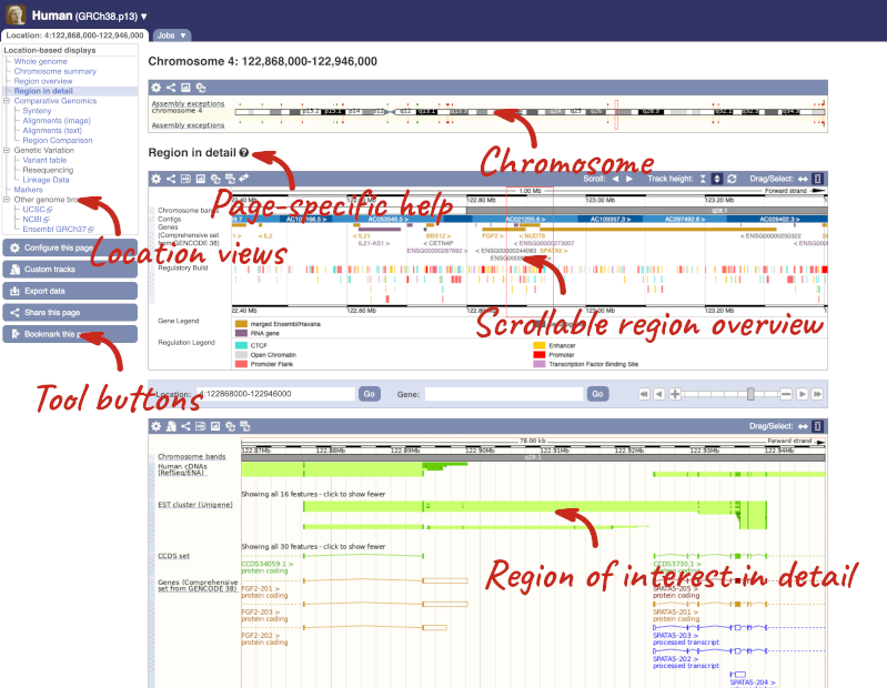
The Region in detail page is made up of three images, let’s look at each one in detail.
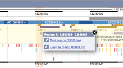
The first image shows the chromosome:
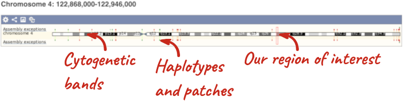
The region we’re looking at is highlighted on the chromosome. You can jump to a different region by dragging out a box in this image. Drag out a box on the chromosome, a pop-up menu will appear.
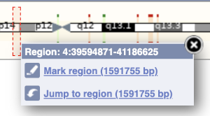
If you wanted to move to the region, you could click on Jump to region (### bp). If you wanted to highlight it, click on Mark region (###bp). For now, we’ll close the pop-up by clicking on the X on the corner.
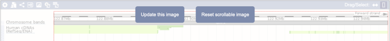
The second image shows a 1Mb region around our selected region. This is always 1Mb in human, but the fixed size of this view varies between species. This view allows you to scroll back and forth along the chromosome.
You can also drag out and jump to or mark a region.
Click on the X to close the pop-up menu.
Click on the Drag/Select button  to change the action of your mouse click. Now you can scroll along the chromosome by clicking and dragging within the image. As you do this you’ll see the image below grey out and two blue buttons appear. Clicking on Update this image would jump the lower image to the region central to the scrollable image. We want to go back to where we started, so we’ll click on Reset scrollable image.
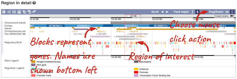
The third image is a detailed, configurable view of the region.
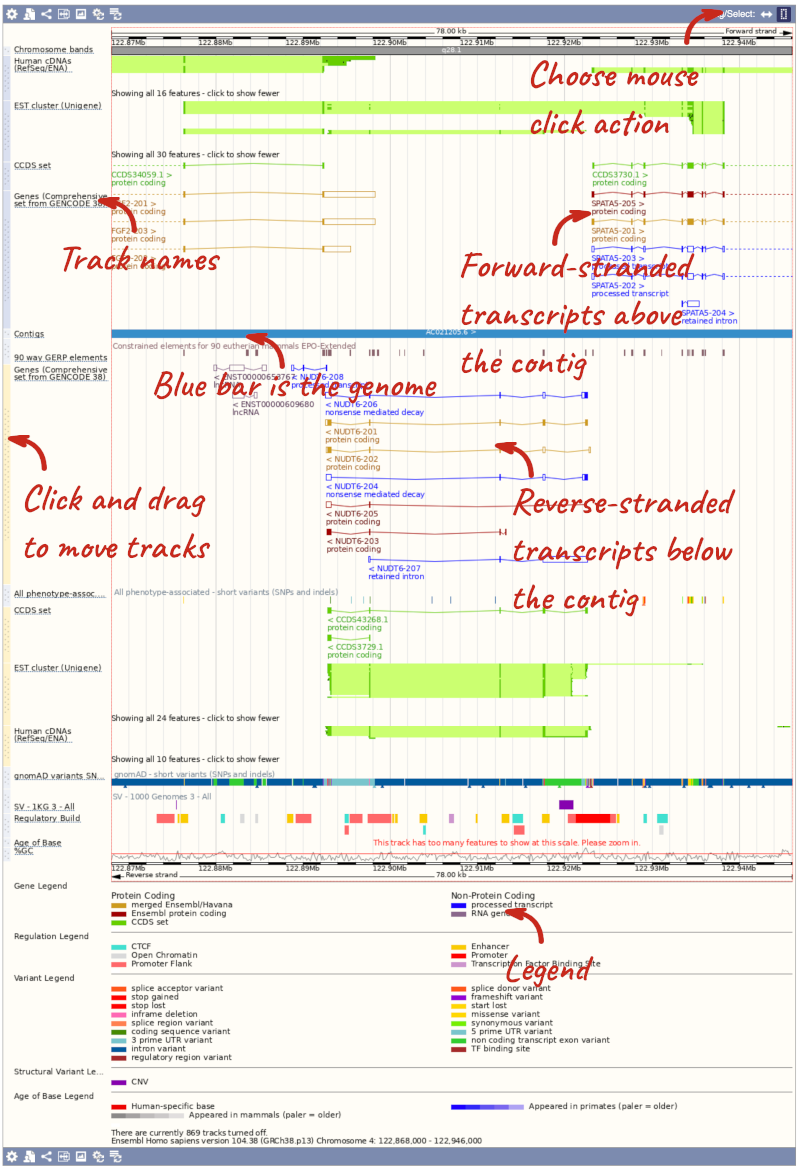
Here you can see various tracks, which is what we call a data type that you can plot against the genome. Some tracks, such as the transcripts, can be on the forward or reverse strand. Forward stranded features are shown above the blue contig track that runs across the middle of the image, with reverse stranded features below the contig. Other tracks, such as variants, regulatory features or conserved regions, refer to both strands of the genome, and these are shown by default at the very top or very bottom of the view.
You can use click and drag to either navigate around the region or highlight regions of interest, Click on the Drag/Select option at the top or bottom right to switch mouse action. On Drag, you can click and drag left or right to move along the genome, the page will reload when you drop the mouse button. On Select you can drag out a box to highlight or zoom in on a region of interest.
With the tool set to Select, drag out a box around an exon and choose Mark region.
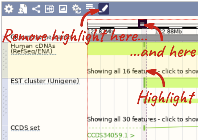
The highlight will remain in place if you zoom in and out or move around the region. This allows you to keep track of regions or features of interest.
We can edit what we see on this page by clicking on the blue Configure this page menu at the left.

This will open a menu that allows you to change the image.
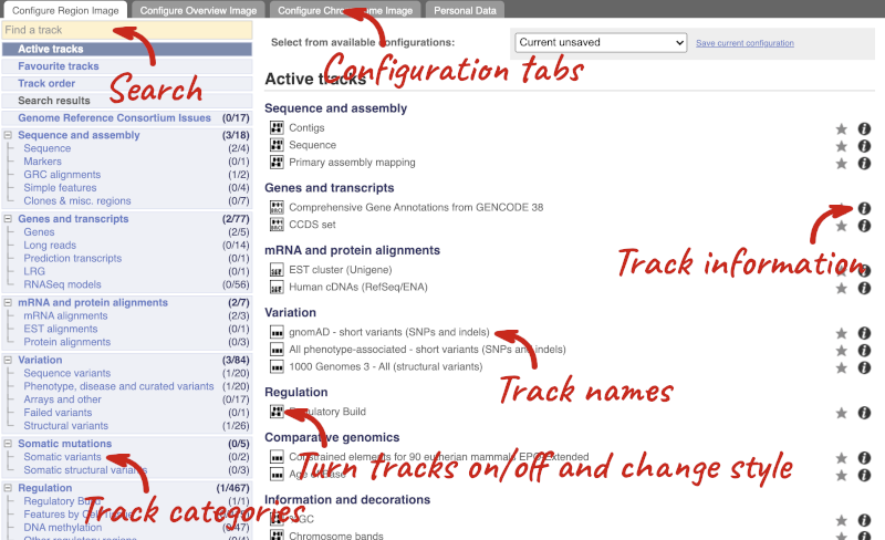
There are thousands of possible tracks that you can add. When you launch the view, you will see all the tracks that are currently turned on with their names on the left and an info icon on the right, which you can click on to expand the description of the track. Turn them on or off, or change the track style by clicking on the box next to the name. More details about the different track styles are in this FAQ: http://www.ensembl.org/Help/Faq?id=335.
You can find more tracks to add by either exploring the categories on the left, or using the Find a track option at the top left. Type in a word or phrase to find tracks with it in the track name or description.
Let’s add some tracks to this image. Add:
- Proteins (mammal) from UniProt – Labels
- 1000 Genomes - All - short variants (SNPs and indels) – Normal
Now click on the tick in the top left hand to save and close the menu. Alternatively, click anywhere outside of the menu. We can now see the tracks in the image. The proteins track is stranded, so you will see two tracks, one above and one below the contig, representing the proteins mapped to the forward and reverse strands respectively. The variants track is not stranded, so is found near the bottom of the image.
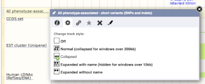
If the track is not giving you can information you need, you can easily change the way the tracks appear by hovering over the track name then the cog wheel to open a menu. To make it easier to compare information between tracks, such as spotting overlaps, you can move tracks around by clicking and dragging on the bar to the left of the track name.
Now that you’ve got the view how you want it, you might like to show something you’ve found to a colleague or collaborator. Click on the Share this page button to generate a link. Email the link to someone else, so that they can see the same view as you, including all the tracks you’ve added. These links contain the Ensembl release number, so if a new release or even assembly comes out, your link will just take you to the archive site for the release it was made on.

To return this to the default view, go to Configure this page and select Reset configuration at the bottom of the menu.
Exploring a genomic region in human
Go to Ensembl.
-
Go to the region from 32,264,000 to 32,492,000 bp on human chromosome 13. On which cytogenetic band is this region located? How many contigs make up this portion of the assembly (contigs are contiguous stretches of DNA sequence that have been assembled solely based on direct sequencing information)?
-
Zoom in on the BRCA2 gene.
-
Configure this page to turn on the LTR (repeat) track in this view. What tool was used to annotate the LTRs according to the track information? How many LTRs can you see within the BRCA2 gene? Do any overlap exons?
-
Create a Share link for this display. Email it to your neighbour. Open the link they sent you and compare. If there are differences, can you work out why?
-
Export the genomic sequence of the region you are looking at in FASTA format.
-
Turn off all tracks you added to the Region in detail page.
- Go to the Ensembl homepage, select Human from the Species drop-down list and type
13:32264000-32492000in the text box (alternatively leave the Search drop-down list as it is and type13:32264000-324920000in the text box). Click Go.This genomic region is located on cytogenetic band q13.1. It is made up of three contigs, indicated by the alternating light and dark blue coloured bars in the Contigs track.
-
Draw with your mouse a box encompassing the BRCA2 transcripts. Click on Jump to region in the pop-up menu.
- Click Configure this page in the side menu (or on the cog wheel icon in the top left hand side of the bottom image). Go into Repeats in the left-hand menu then select LTR. Click on the (i) button to find out more information.
Repeat Masker was used to annotate LTRs onto the genome.
Save and close the new configuration by clicking on ✓ (or anywhere outside the pop-up window). There are ten LTRs overlapping BRCA2, none of them overlap exons. -
Click Share this page in the side menu. Copy the URL. Get your neighbour’s email address and compose an email to them, paste the link in and send the message. When you receive the link from them, open the email and click on your link. You should be able to view the page with the new configuration and data tracks they have added to in the Location tab. You might see differences where they specified a slightly different region to you, or where they have added different tracks.
Here is the Share link from the video answer: https://may2021.archive.ensembl.org/Homo_sapiens/Share/71a173bba78f0dbe03e48d3240424943?redirect=no;mobileredirect=no
-
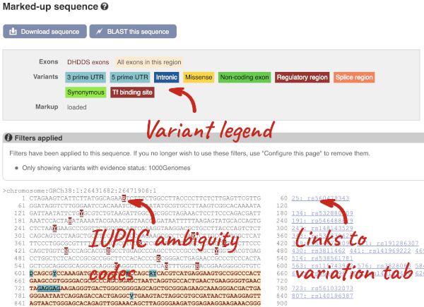
Click Export data in the side menu. Leave the default parameters as they are (FASTA sequence should already be selected). Click Next>. Click on Text. Note that the sequence has a header that provides information about the genome assembly (GRCh38), the chromosome, the start and end coordinates and the strand. For example:
>13_dna:chromosome_chromosome:GRCh38:13:32311910:32405865:1 - Click Configure this page in the side menu. Click Reset configuration. Click ✓.
Exploring a genomic region in mouse
Go to the Ensembl homepage.
-
Go to the region from 150,320,000 to 150,540,000 bp on mouse chromosome 5. How many contigs make up this portion of the assembly (contigs are contiguous stretches of DNA sequence that have been assembled solely based on direct sequencing information)?
-
Zoom in on the Brca2 gene.
-
Configure this page to turn on the LTR (repeat) track in this view. What tool was used to annotate the LTRs according to the track information? How many LTRs can you see within the Brca2 gene? Do any overlap exons?
-
Create a Share link for this display. Email it to your neighbour. Open the link they sent you and compare. If there are differences, can you work out why?
-
Export the genomic sequence of the region you are looking at in FASTA format.
-
Turn off all tracks you added to the Region in detail page.
- Select Mouse from the Species search list and type
5:150320000-150540000in the text box (or alternatively leave the Search drop-down list like it is and typemouse 5:150320000-150540000in the text box). Click Go.It is made up of five contigs, indicated by the alternating light and dark blue coloured bars in the Contigs track. Note the tiny contig, AEKQ02165236.1, which splits AC084217.7 in two.
-
Draw with your mouse a box encompassing the Brca2 transcripts. Click on Jump to region in the pop-up menu.
- Click Configure this page in the side menu (or on the cog wheel icon in the top left hand side of the bottom image). Go to Repeats in the left-hand menu then select LTRs (Repeats (Mouse)). Click on the (i) button to find out more information.
Repeat Masker was used to annotate LTRs onto the genome.
Save and close the new configuration by clicking on ✓ (or anywhere outside the pop-up window).
There are seven LTRs overlapping Brca2, none of them overlap exons.
-
Click Share this page in the side menu. Select the link and copy. Get your neighbour’s email address and compose an email to them, paste the link in and send the message. When you receive the link from them, open the email and click on your link. You should be able to view the page with the new configuration and data tracks they have added to in the Location tab. You might see differences where they specified a slightly different region to you, or where they have added different tracks.
-
Click Export data in the side menu. Leave the default parameters as they are. Click Next>. Click on Text.
- Click Configure this page in the side menu. Click Reset configuration. Click ✓.
Exploring a genomic region in Oryza sativa Japonica (rice)
Go to the Ensembl Plants homepage and do the following:
-
Go to the region between 405000 and 453000 on chromosome 1 in Oryza sativa Japonica.
-
Turn on the AGILENT:G2519F-015241 microarray track. Are there any oligo probes that map to this region?
-
Highlight the region around any reverse strand probes you can see. Do they map to any Ensembl transcripts?
-
Go to the Ensembl Plants homepage. Select Oryza sativa Japonica from the Species drop-down list and type
1:405000-453000. Click Go. - Click on Configure this page to open the menu. You can find the AGILENT:G2519F-015241 track under Oligo probes in the left-hand menu, or by using the Find a track box at the top right. Turn on the track as Normal then save and close the menu. As the AGILENT:G2519F-015241 track is stranded, it appears at the top and bottom of the view.
There are 5 probes mapped to this region on the positive strand and one probe on the reverse strand.
- Drag a box around the reverse strand probe then click on Mark region to highlight.
The highlighted region maps to two transcripts: Os01t0107900-02 and Os01t0107900-01
Exploring a region in Coprinopsis cinerea okayama
Go to Ensembl Fungi. Let’s try to find some information about the region from 1,400,000 to 1,425,000 in chromosome 7 in Coprinopsis cinerea okayama:
-
How many complete genes are found in this region? How many on the forward and how many on the reverse strand?
-
Zoom in on the largest gene EFI27358. How many exons does this gene have?
-
Export the genomic sequence in FASTA format for this region.
- In the Ensembl Fungi homepage, select Coprinopsis cinerea okayama from the Species search drop-down. Enter
7:1400000-1425000in the Search bar and click Go. This will send you to the Location tab. Your region of interest is indicated by a red rectangle in the 50kb view. Look at the Genes track: each block represents a different gene. Count the number of complete genes within the rectangle.There are 7 complete genes in the region.
- Look at the Region in detail view (the most detailed view at the bottom of the page). You can zoom into a region by clicking and dragging your mouse (you can change your mouse action in the top right-hand corner of the view under **Drag/Select) and selecting Jump to region in the pop-up menu. Count the number of blocks you can see for EFI27358.
The EFI27358 gene has 23 exons.
Click on the transcript ID CZT99117 in the transcript table.
It has 4 exons.
- We want to export the genomic sequence for our original region (not just the EFI27358 gene). You can reset the view by entering
7:1400000-1425000in the Location bar above the Region in detail view or hitting the Back button on your internet browser. Click on Export data in the left-hand panel. In the pop-up menu, select FASTA from the drop-down and click Next >. You can export the sequence as is (text) or as a compressed file (.gz).If you choose to download the sequence as text, your browser might open the FASTA file in a new tab. In this case, just right-click on any white space and select Save As… from the menu.
Exploring a genomic region in Salmonella enterica
Go to Ensembl Bacteria and do the following:
-
Search for the Salmonella enterica subsp. enterica serovar Typhi str. Ty2 (GCA_000007545) (Hint: type
Tyinto the Search for a genome box). -
Go to the region Chromosome:2000605-2009742.
-
How many genes are annotated in this region? How many are on the forward strand? How many are on the reverse strand?
-
Go to the Ensembl Bacteria homepage. Type
Ty2into the Search for a genome box. Click on the auto-completed genome name to navigate to the species information page. -
Type
Chromosome:2000605-2009742into the search box. Click Go. -
There are 8 genes annotated in this region, all on the reverse strand.
Variation
In any of the sequence views shown in the Gene and Transcript tabs, you can view variants on the sequence. You can do this by clicking on Configure this page from any of these views.
Let’s take a look at the Gene sequence view for HBB in human. Search for HBB and go to the Sequence view.
If you can’t see variants marked on this view, click on Configure this page and select Show variants: Yes and show links. You may also wish to add a filter to the variants to allow them to load more quickly, we’ll add Filter variants by evidence status: 1000Genomes.
Find out more about a variant by clicking on it.
You can add variants to all other sequence views in the same way.
You can go to the Variation tab by clicking on the variant ID. For now, we’ll explore more ways of finding variants.
To view all the sequence variants in table form, click the Variant table link at the left of the gene tab.
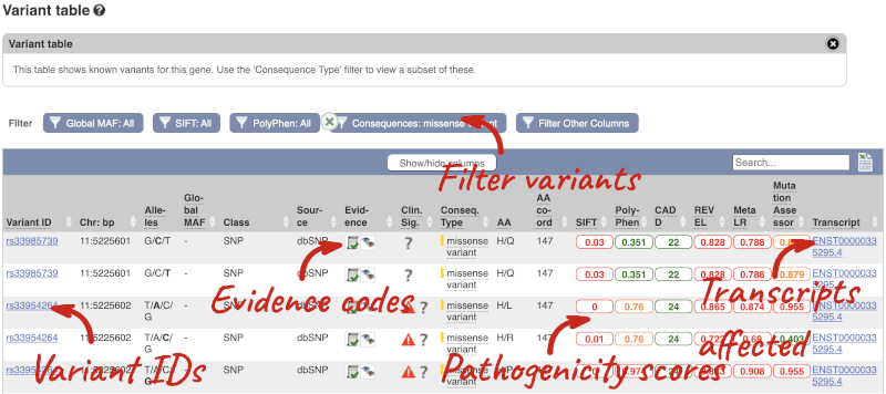
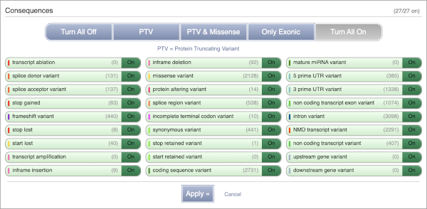
You can filter the table to only show the variants you’re interested in. For example, click on Consequences: All, then select the variant consequences you’re interested in. For display purposes, the table above has already been filtered to only show missense variants.
You can also filter by the different pathogenicity scores and MAF, or click on Filter other columns for filtering by other columns such as Evidence or Class.
The table contains lots of information about the variants. You can click on the IDs here to go to the Variation tab too.
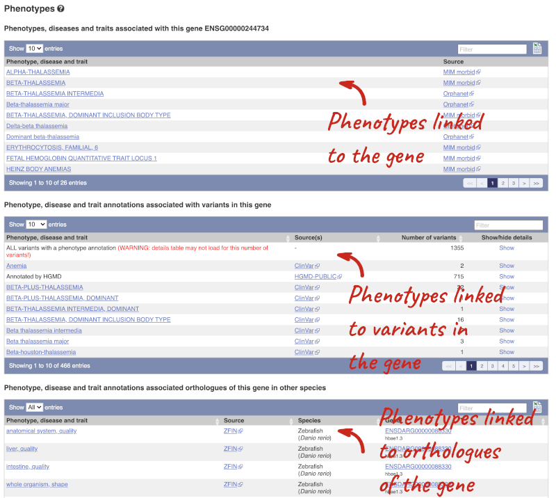
You can also see the phenotypes associated with a gene. Click on Phenotype in the left hand menu.
Open the transcript table and go to HBB-201 ENST00000335295, then click on Haplotypes in the left hand menu.
![]()
The Haplotypes view in the transcript tab shows you the actual protein and CDS sequences in 1000 Genomes individuals. This is possible because the 1000 Genomes study has phased genotypes, so we know which alleles occur on which of the chromosome pairs. The table lists all the versions of the protein that occur along with their frequencies, including the reference sequence and sequences with one or more alternative alleles.
Click on one of the haplotypes, we’ll go for 18K>*,19del{130}, to find out more about it. Here you will see the frequency in the 1000 Genomes subpopulations, the sequence and the 1000 Genomes individuals where this protein is found.
Let’s have a look at variants in the Location tab. Click on the Location tab in the top bar.
Configure this page and open Variation from the left-hand menu.
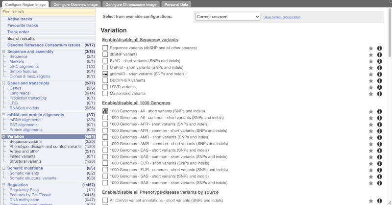
There are various options for turning on variants. You can turn on variants by source, by frequency, presence of a phenotype or by individual genome they were isolated from. You can also turn on genotyping chips.
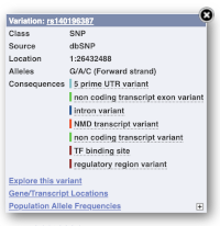
Let’s have a look at a specific variant. If we zoomed in we could see the variant rs334 in this region, however it’s easier to find if we put rs334 into the search box. Click through to open the Variation tab.
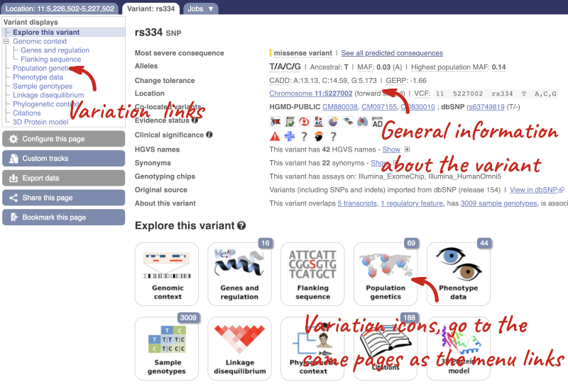
The icons show you what information is available for this variant. Click on Genes and regulation, or follow the link on the left.
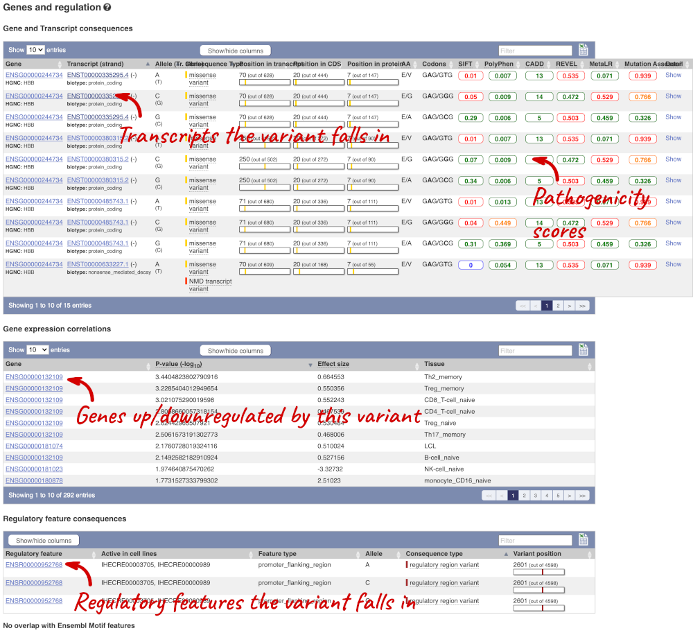
This page illustrates the genes the variant falls within and the consequences on those genes, including pathogenicity predictors. It also shows data from GTEx on genes that have increased/decreased expression in individuals with this variant, in different tissues. Finally, regulatory features and motifs that the variant falls within are shown.
We can also see the variant in the protein structure by clicking on 3D Protein model.
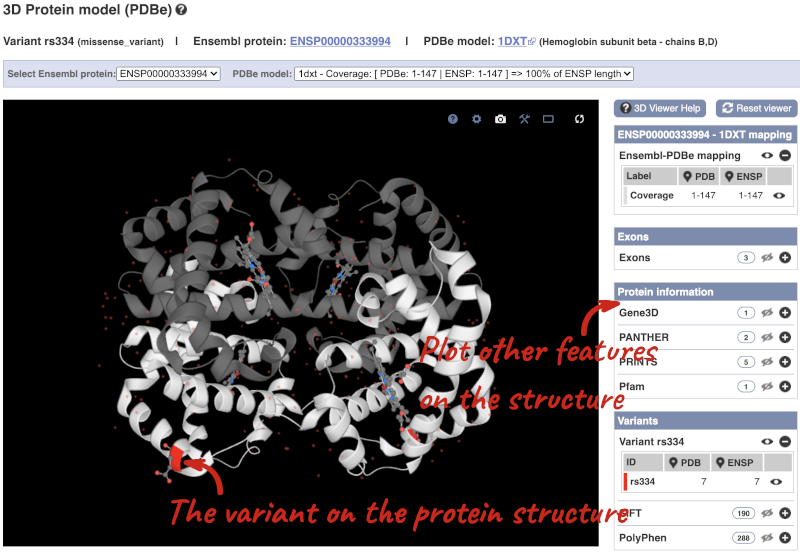
This is a LiteMol viewer, where you can rotate and zoom in on the structure. The variant location is highlighted, so you can see where it lands within the structure.
Let’s look at population genetics. Click on Population genetics in the left-hand menu.
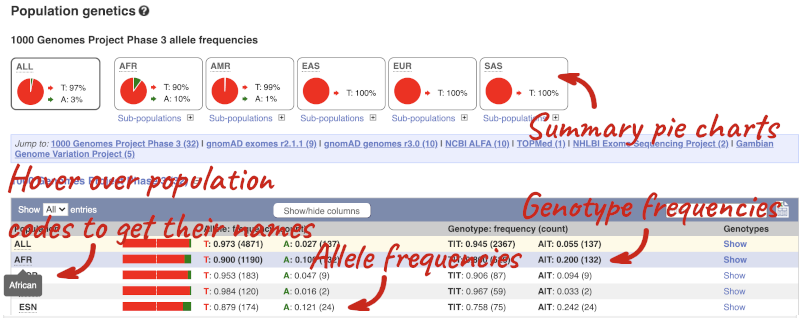
The population allele frequencies are shown by study, including 1000 Genomes and gnomAD. Where genotype frequencies are available, these are shown in the tables.
There are big differences in allele frequencies between populations. Let’s have a look at the phenotypes associated with this variant to see if they are known to be specific to certain human populations. Click on Phenotype Data in the left-hand menu.
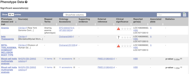
This variant is associated with various phenotypes, including sickle cell and malaria resistance. These phenotype associations come from sources including the GWAS catalog, ClinVar, Orphanet and OMIM. Where available, there are links to the original paper that made the association, the allele that is associated with the phenotype and p-values and other statistics.
Human population genetics and phenotype data
The SNP rs1738074 in the 5’ UTR of the human TAGAP gene has been identified as a genetic risk factor for a few diseases. Use Ensembl to answer the following questions:
-
In which transcripts is this SNP found?
-
What is the least frequent genotype for this SNP in the Yoruba (YRI) population from the 1000 Genomes phase 3?
-
What is the ancestral allele? Is it conserved in the 91 eutherian mammals EPO-Extended?
-
With which diseases is this SNP associated? Are there any known risk (or associated) alleles?
- Please note there is more than one way to get this answer. Either go to the Variation table of the human TAGAP gene, and use the Consequence filter to only include 5’UTR variants, or search Ensembl for
rs1738074directly. Once you’re in the Variant tab, click on Genes and regulation in the menu.This SNP is found in four transcripts of TAGAP. It is also an intron_variant to one lncRNA transcript of TAGAP-AS1.
- Click on Population genetics in the left-hand panel, or click on Explore this variant in the left-hand panel and click the Population genetics icon.
In Yoruba (YRI), the least frequent genotype is CC at the frequency of 5.6%.
- Click on Phylogenetic context in the left-hand panel.
The ancestral allele is T and it’s inferred from the alignment in primates.
Click on Select an alignment which will open a pop-up menu. Open Multiple alignments and select 91 eutherian mammals EPO-Extended. Click on Apply at the bottom of the menu to save your settings.
A region containing the SNP (highlighted in red and placed in the centre) and its flanking sequence are displayed. The T allele is conserved in all but two of the eutherian mammals displayed.
- Click Phenotype data in the left-hand panel.
This variation is associated with multiple sclerosis, celiac disease and white blood cell count. There are known risk alleles for all three diseases and the corresponding P values are provided. The allele A is associated with celiac disease. Note that the alleles reported by Ensembl are T/C. Ensembl reports alleles on the forward strand. This suggests that A was reported on the reverse strand in the original paper. Similarly, one of the alleles reported for Multiple sclerosis is G.
Exploring VNTR in human
Variable number tandem repeats (VNTRs) show high variation in the number of repeats in the population and are commonly used in forensics (DNA fingerprinting) and to study genetic diversity. (a) Go to the region from 3074666 to 3075100 bp on human chromosome 4. Which gene does it overlap? Which exon of this gene falls in this region?
(b) Configure this page to turn on Repeats (low), Simple repeats (Repeats (low)) and Tandem repeats (TRF) tracks in this view. Can you see any repeats in this exon? What tools were used to annotate the repeats according to the track information?
(c) Zoom in on the (CAG)n to see its sequence. How many CAG repeats can you see in the human reference assembly? Does this track overlap any phenotype-associated variants? What is the identifier of this variant?
(d) Go to the variant tab of the phenotype-associated variant. What is the consequence ontology of this variant? Does the reference allele match the number of repeats you have just counted? What is the shortest and longest allele?
(a) Select Search: Human and type 4:3074666-3075100 in the text box (or alternatively type human 4:3074666-3075100 in the text box). Click Go.
Click on the golden transcript falling in this region. You can see it’s exon 1 of 67 of the huntingtin gene (HTT).
(b) Click Configure this page in the side menu then select: Repeats (low), Simple repeats (Repeats (low)) and Tandem repeats (TRF).
There are three tandem repeats in this exon, and two simple repeats (low); (CAG)n and (CCG)n. Click on the track names to find more about the tools used for annotation: RepeatMasker and Tandem Repeats Finder.
(c) Draw with your mouse a box around the (CAG)n repeat. Click on Jump to region in the pop-up menu.
There are 19 CAG repeats in the human reference sequence overlapping rs71180116 indicated by a pink bar in the All phenotype-associated - short variants (SNPs and indels) track.
(d) Click on the rs71180116 ID to go to the variant tab. You can see in the summary page that this variant is classified as an inframe insertion. Either click + to show all of the alleles in the summary page or go to the Genes and regulation table. This variant has many alternative alleles which differ in the number of repeats. The first allele in the expanded Alleles section of the summary page or the first allele in the Codons column in the Genes and regulation table is the reference allele. It is composed of 19 CAG repeats just as in the Region in detail view. The shortest allele has 7 repeats, the longest has 55 repeats.
Exploring a SNP in mouse
In the paper “Altered metabolic signature in pre-diabetic NOD mice” (PloS One. 2012; 7(4): e35445), Madsen et al. have described several regulatory and coding SNPs, some of them in genes involved in ATP and adenosine metabolism, leading to potentially faulty metabolism of ATP and adenosine. The authors describe that one of the identified SNPs in the murine Entpd2 gene (rs28232063) would lead to increased amounts of available ATP, an immune activator, causing increased cell activation and possibly autoreactive T-cell activation. Use Ensembl to answer the following questions:
-
Where is the SNP located (chromosome and coordinates)?
-
What is the HGVS recommendation nomenclature for this SNP?
-
Why does Ensembl put the G allele first (G/A)?
-
Are there differences between the genotypes reported in C57BL/6NJ and NOD/ShiLtJ, according to the Mouse Genomes Project?
- From the Ensembl homepage, select Mouse from the Species search drop-down and enter
rs28232063in the search box.SNP rs28232063 is located on 2:25288362. In Ensembl, its alleles are provided relative to the forward strand.
- Click on Show under HGVS names to reveal information about HGVS nomenclature.
This SNP has got four HGVS names, one at the genomic DNA level (NC_000068.8:g.25288362G>A), two at the transcript level (ENSMUST00000148859.2:n.444-182G>A and ENSMUST00000028328.3:c.446G>A) and one at the protein level (ENSMUSP00000028328.3:p.Arg149Gln).
- In Ensembl, the allele that is present in the reference genome assembly is always put first.
G is the allele for the reference mouse genome strain C57BL/6J
- Click on Sample genotypes is the left-hand panel. The table shows genotypes reported for different mouse strains from the Mouse Genomes Project.
There are indeed differences between the genotypes reported in those two different strains. The genotype reported in C57BL/6NJ is G/G whereas in NOD/ShiLtJ the genotype is A/A.
Variation data in tomato
-
Go to Ensembl Plants and find the Solyc02g084570.3 gene in Solanum lycopersicum (tomato) and go to its Location tab. Can you see the variation track?
-
Zoom in around the last exon of this gene. What are the different types of variants seen in that region? Are any splice region variants mapped in the region? If so, what is/are the coordinate(s)?
- Select Solanum lycopersicum from the Species search drop-down menu and search for
Solyc02g084570.3. In the results page, you can click on the coordinates 2:48284598-48288482 to go straight to the Location tab. Scroll down to the Region in detail view. The variation track is shown at the bottom of the view.If you don’t see the Variation - All sources track, click Configure this page on the left-hand panel, search for the track in the pop-up menu and enable the track by clicking on the square next to the track name. Close the pop-up window and wait for the track to load.
- Zoom in around the last exon of this gene by drawing a box in the respective region (you can change your mouse action by clicking the Drag/Select icons at the top right-hand corner of the view). Note the gene is on the reverse strand (this is signified by the < sign next to the transcript name, and it is located below the Contigs track), so the last exon will be on the left hand side of that image. The variation legend is shown at the bottom of the page, telling you what the colours mean.
The types of variants seen in that region are 3’ UTR, missense, synonymous and splice region variants.
Splice region variants are shown in orange. Click on the variants to get additional information on that variant including location. You can zoom into the region if the variant block is too small to click.
The variants are found at 2:48285642 and 2:48285640-48285641. Note that the two variants overlap: one is a SNP and the other is an indel. SNPs are tagged with ambiguity codes (zoom into the region if you cannot see this). You can find a useful IUPAC ambiguity code guid on the bioinformatics.org website. Single-letter ambiguity codes are given when two or more possible nucleotides may be represented at a single base locus.
Variation data in Fusarium oxysporum
-
How many species in Ensembl Fungi have variation data?
-
Select Fusarium oxysporum (FO2) and search for the FOXG_13574T0 gene. One of its upstream variants is SNP tmp_10_6610. What are the possible alleles for this polymorphic position? Which one is on the reference genome?
-
What is the most frequent allele at this position?
-
Which samples have the genotypes C|T and T|T?
- Go to Ensembl Fungi, click on View full list of all species. You can sort the table by column. Click on the Variation database column to sort the table by species with variation data.
The table shows that we have 8 fungi species currently with variation databases.
- Click on Fusarium oxysporum in the table and on the species page search for
FOXG_13574T0. From the Gene tab, click on Variant table in the left-hand panel. You can use the filter at the top right-hand corner of the tabletmp_10_6610.The alleles are C/T, where C is the reference allele.
- Click on tmp_10_6610 in the table to open the Variant tab. Then click on Genotype frequency from the menu on the left-hand side of the page.
The most frequent allele at this position is C with a frequency of 0.850.
- Click on Sample genotypes in the menu on the left.
The table shows that sample 909454 has the C|T genotype and 909455 has the T|T genotype.
VEP
We have identified five variants on human chromosome nine, C-> A at 128203516, an A deletion at 128328461, C->A at 128322349, C->G at 128323079 and G->A at 128322917.
We will use the Ensembl VEP to determine:
- Have my variants already been annotated in Ensembl?
- What genes are affected by my variants?
- Do any of my variants affect gene regulation?
Go to the front page of Ensembl and click on the Variant Effect Predictor.
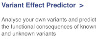
This page contains information about the VEP, including links to download the script version of the tool. Click on Launch VEP to open the input form:
The data is in VCF format:
chromosome coordinate id reference alternative
Put the following into the Paste data box:
9 128328460 var1 TA T
9 128322349 var2 C A
9 128323079 var3 C G
9 128322917 var4 G A
9 128203516 var5 C A
The VEP will automatically detect that the data is in VCF.
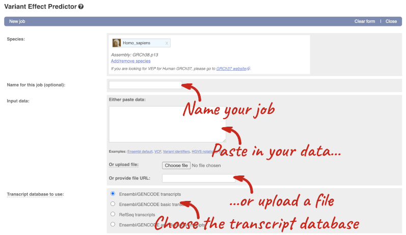
There are further options that you can choose for your output. These are categorised as Identifiers, Variants and frequency data, Additional annotations, Predictions, Filtering options and Advanced options. Let’s open all the menus and take a look.
Hover over the options to see definitions.
We’re going to select some options:
- HGVS, annotation of variants in terms of the transcripts and proteins they affect, commonly-used by the clinical community
- Phenotypes
- Protein domains
When you’ve selected everything you need, scroll right to the bottom and click Run.
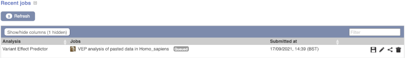
The display will show you the status of your job. It will say Queued, then automatically switch to Done when the job is done, you do not need to refresh the page. You can edit or discard your job at this time. If you have submitted multiple jobs, they will all appear here.
Click View results once your job is done.
In your results you will see a graphical summary of your data, as well as a table of your results.
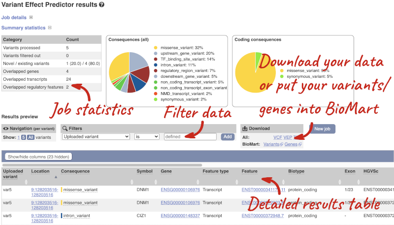
The results table is enormous and detailed, so we’re going to go through the it by section. The first column is Uploaded variant. If your input data contains IDs, like ours does, the ID is listed here. If your input data is only loci, this column will contain the locus and alleles of the variant. You’ll notice that the variants are not neccessarily in the order they were in in your input. You’ll also see that there are multiple lines in the table for each variant, with each line representing one transcript or other feature the variant affects.
You can mouse over any column name to get a definition of what is shown.
The next few columns give the information about the feature the variant affects, including the consequence. Where the feature is a transcript, you will see the gene symbol and stable ID and the transcript stable ID and biotype. Where the feature is a regulatory feature, you will get the stable ID and type. For a transcription factor binding motif (labelled as a MotifFeature) you will see just the ID. Most of the IDs are links to take you to the gene, transcript or regulatory feature homepage.
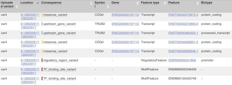
This is followed by details on the effects on transcripts, including the position of the variant in terms of the exon number, cDNA, CDS and protein, the amino acid and codon change, transcript flags, such as MANE, on the transcript, which can be used to choose a single transcript for variant reporting, and predicted pathogenicity scores. The predicted pathogenicity scores are shown as numbers with coloured highlights to indicate the prediction, and you can mouse-over the scores to get the prediction in words. Two options that we selected in the input form are the HGVS notation, which is shown to the left of the image below and can be used for reporting, and the Domains to the right. The Domains list the proteins domains found, and where there is available, provide a link to the 3D protein model which will launch a LiteMol viewer, highlighting the variant position.
![]()
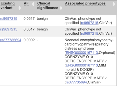
Where the variant is known, the ID of the existing variant is listed, with a link out to the variant homepage. In this example, only rsIDs from dbSNP are shown, but sometimes you will see IDs from other sources such as COSMIC. The VEP also looks up the variant from frequency files, and pulls back the allele frequency (AF in the table), which will give you the 1000 Genomes Global Allele Frequency. In our query, we have not selected allele frequencies from the continental 1000 Genomes populations or from gnomAD, but these could also be shown here. We can also see ClinVar clinical significance and the phenotypes associated with known variants or with the genes affected by the variants, with the variant ID listed for variant associations and the gene ID listed for gene associations, along with the source of the association.
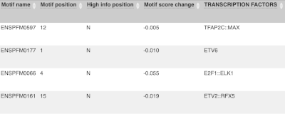
For variants that affect transcription factor binding motifs, there are columns that show the effect on motifs (you may need to click on Show/hide columns at the top left of the table to display these). Here you can see the position of the variant in the motif, if the change increases or decreases the binding affinity of the motif and the transcription factors that bind the motif.
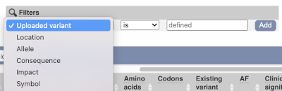
Above the table is the Filter option, which allows you to filter by any column in the table. You can select a column from the drop-down, then a logic option from the next drop-down, then type in your filter to the following box. We’ll try a filter of Consequence, followed by is then missense_variant, which will give us only variants that change the amino acid sequence of the protein. You’ll notice that as you type missense_variant, the VEP will make suggestions for an autocomplete.
You can export your VEP results in various formats, including VCF. When you export as VCF, you’ll get all the VEP annotation listed under CSQ in the INFO column. After filtering your data, you’ll see that you have the option to export only the filtered data. You can also drop all the genes you’ve found into the Gene BioMart, or all the known variants into the Variation BioMart to export further information about them.
Running CFTR variants through VEP
Resequencing of the genomic region of the human CFTR (cystic fibrosis transmembrane conductance regulator (ATP-binding cassette sub-family C, member 7) gene (ENSG00000001626) has revealed the following variants. The alleles defined in the forward strand:
- G/A at 7: 117,530,985
- T/C at 7: 117,531,038
- T/C at 7: 117,531,068
Use the VEP tool in Ensembl and choose the options to see SIFT and PolyPhen predictions. Do these variants result in a change in the proteins encoded by any of the Ensembl genes? Which gene? Have the variants already been found?
Go to the Ensembl homepage and click on the link Tools at the top of the page. Currently there are nine tools listed in that page. Click on Variant Effect Predictor and enter the three variants as below:
7	117530985	117530985	G/A
7	117531038	117531038	T/C
7	117531068	117531068	T/C
Note: Variation data input can be done in a variety of formats. See more details about the different data formats and their structure in this VEP documentation page. Click Run. When your job is listed as Done, click View Results.
You will get a table with the consequence terms from the Sequence Ontology project (http://www.sequenceontology.org/) (i.e. synonymous, missense, downstream, intronic, 5’ UTR, 3’ UTR, etc) provided by VEP for the listed SNPs. You can also upload the VEP results as a track and view them on Location pages in Ensembl. SIFT and PolyPhen are available for missense SNPs only. For two of the entered positions, the variations have been predicted to have missense consequences of various pathogenicity (coordinate 117531038 and 117531068), both affecting CFTR. All the three variants have been already annotated and are known as rs1800077, rs1800078 and rs35516286 in dbSNP (databases, literature, etc).
VEP analysis of structural variants in human
We have details of a genomic deletion in a breast cancer sample in VCF format:
13 32307062 sv1 . <DEL> . . SVTYPE=DEL;END=32908738
Use VEP in Ensembl to find out the following information:
1. How many genes have been affected?
2. Does the structural variant (SV) cause deletion of any complete transcripts?
3. Map your variant in the Ensembl browser on the Region in detail view.
- Click on VEP at the top of any Ensembl page and open the web interface. Make sure your species is Human. It is good practise to name your VEP jobs something descriptive, such as Patient deletion exercise. Paste the variant in VCF format into the Paste data field and hit Run.
12 different genes are affected by the SV.
- Filter your table by select Consequence is
transcript_ablationat the top of the table and click Add.Yes, there is deletion of complete transcripts of PDS5B, N4BP2L1, BRCA2, RNY1P4, IFIT1P1, ATP8A2P2, N4BP2L2, N4BP2L2-IT2 and one gene without official symbols: ENSG00000212293.
- To view your variant in the browser click on the location link in the results table 13: 32307062-32908738. The link will open the Region in detail view in a new tab. If you have given your data a name it will appear automatically in red. If not, you may need to Configure this page and add it under the Personal data tab in the pop-up menu.