Filter Events by Year
Ensembl Browser Workshop: Plant & Animal Genome Conference (PAG) 31
Course Details
- Lead Trainer
- Adam Frankish
- Associate Trainer(s)
- Event Date
- 2024-01-14
- Location
- Town and Country D, Town & Country Resort and Conference Center, San Diego, CA 92108
- Description
- Work with the Ensembl Outreach team to get to grips with the Ensembl browser, accessing gene, variation, comparative genomics and regulation data, and mine these data with BioMart.
Demos and exercises
Exploring genomic regions
Demo: Exploring genomic regions in Ensembl Plants
Start at the Ensembl Plants front page. You can search for a region by typing it into a search box, but you have to specify the species.
To bypass the text search, you need to input your region coordinates in the correct format, which is chromosome, colon, start coordinate, dash, end coordinate, with no spaces for example: 1D:41289600-41345600. Choose Triticum aestivum from the species drop-down, then type (or copy and paste) these coordinates into the search box.

Press Enter or click Go to jump directly to the Region in detail Page.
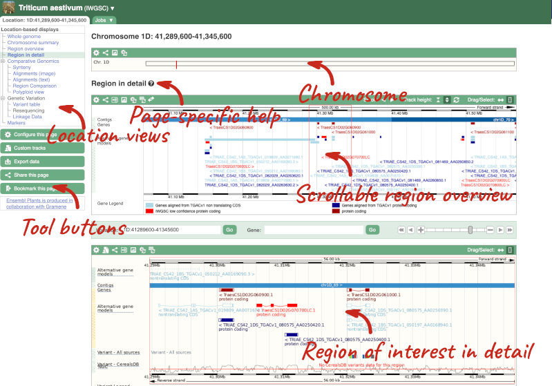
Click on the  button to view page-specific help. The help pages provide text, labelled images and, in some cases, help videos to describe what you can see on the page and how to interact with it.
The Region in detail page is made up of three images, let’s look at each one in detail.
- The first image shows the chromosome:

The region we’re looking at is highlighted on the chromosome. You can jump to a different region by dragging out a box in this image. Drag out a box on the chromosome, a pop-up menu will appear.
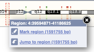
If you wanted to move to the region, you could click on Jump to region (### bp). If you wanted to highlight it, click on Mark region (###bp). For now, we’ll close the pop-up by clicking on the X in the corner.
- The second image shows a 1Mb region around our selected region. This is always 1Mb in human, but the fixed size of this view varies between species. This view allows you to scroll back and forth along the chromosome.
You can also drag out and jump to or mark a region.
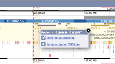
Click on the X to close the pop-up menu.
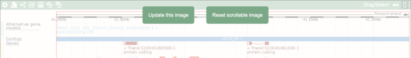
Click on the Drag/Select button  to change the action of your mouse click. Now you can scroll along the chromosome by clicking and dragging within the image. As you do this you’ll see the image below grey out and two blue buttons appear. Clicking on Update this image would jump the lower image to the region central to the scrollable image. We want to go back to where we started, so we’ll click on Reset scrollable image.
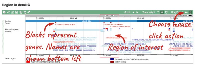
- The third image is a detailed, configurable view of the region.
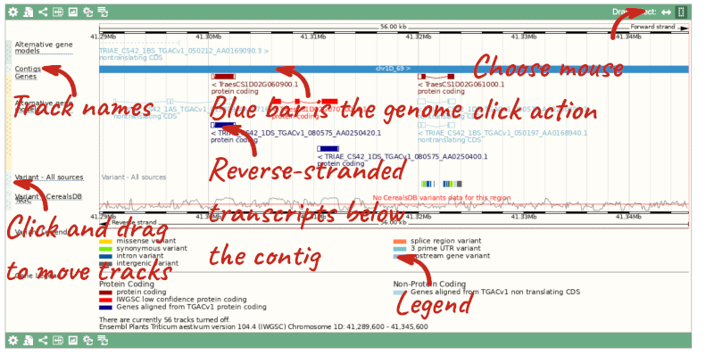
Here you can see various tracks, which is what we call a data type that you can plot against the genome. Some tracks, such as the transcripts, can be on the forward or reverse strand. Forward stranded features are shown above the blue contig track that runs across the middle of the image, with reverse stranded features below the contig. Other tracks, such as variants, regulatory features or conserved regions, refer to both strands of the genome, and these are shown by default at the very top or very bottom of the view.
You can use click and drag to either navigate around the region or highlight regions of interest, Click on the Drag/Select option at the top or bottom right to switch mouse action. On Drag, you can click and drag left or right to move along the genome, the page will reload when you drop the mouse button. On Select you can drag out a box to highlight or zoom in on a region of interest.
With the tool set to Select, drag out a box around an exon and choose Mark region.
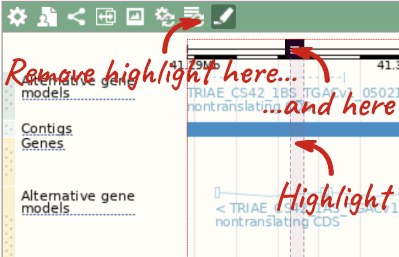
The highlight will remain in place if you zoom in and out or move around the region. This allows you to keep track of regions or features of interest.
We can edit what we see on this page by clicking on the blue Configure this page menu at the left.

This will open a menu that allows you to change the image.
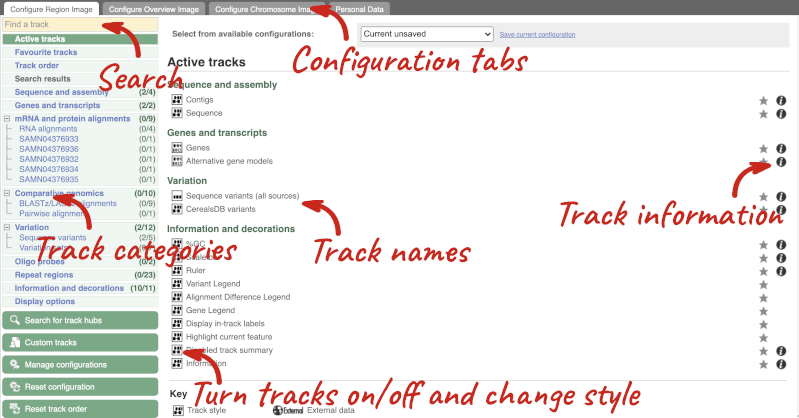
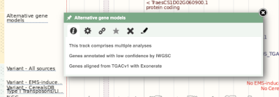
There are thousands of possible tracks that you can add. When you launch the view, you will see all the tracks that are currently turned on with their names on the left and an info icon on the right, which you can click on to expand the description of the track. Turn them on or off, or change the track style by clicking on the box next to the name. More details about the different track styles are in this FAQ.
You can find more tracks to add by either exploring the categories on the left, or using the Find a track option at the top left. Type in a word or phrase to find tracks with it in the track name or description.
Let’s add some tracks to this image. Add:
- EMS-induced mutation variants
- Type I Transposons/LINE (Repeats: Repbase)
Now click on the tick in the top left hand to save and close the menu. Alternatively, click anywhere outside of the menu. We can now see the tracks in the image.
If the track is not giving you can information you need, you can easily change the way the tracks appear by hovering over the track name then the cog wheel to open a menu. To make it easier to compare information between tracks, such as spotting overlaps, you can move tracks around by clicking and dragging on the bar to the left of the track name.
Now that you’ve got the view how you want it, you might like to show something you’ve found to a colleague or collaborator. Click on the Share this page button to generate a link. Email the link to someone else, so that they can see the same view as you, including all the tracks you’ve added. These links contain the Ensembl release number, so if a new release or even assembly comes out, your link will just take you to the archive site for the release it was made on.

To return this to the default view, go to Configure this page and select Reset configuration at the bottom of the menu.
Due to hybridisations in wheat’s evolutionary history, it has a hexaploid genome with related homoeologous regions. We can compare these with the Polyploid view. First, let’s zoom in on the gene TraesCS1D02G061000 by dragging out a box around it and clicking on Jump to region. Now click on the Polyploid view link in the left-hand menu.
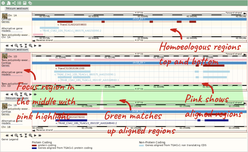
This view also allows us to configure the page, as we could with the main region view, so that we can compare other features between the homoeologous chromosomes.
Demo: Exploring genomic regions in Ensembl Metazoa
We’re going to look at a region of the Anopheles gambiae (African malaria mosquito, PEST) genome, 3L:17000000-17100000, and manipulate the view to see the data we are interested in.


Exploring genomic regions
Demo: Exploring genomic regions in Ensembl Plants
Start at the Ensembl Plants front page. You can search for a region by typing it into a search box, but you have to specify the species.
To bypass the text search, you need to input your region coordinates in the correct format, which is chromosome, colon, start coordinate, dash, end coordinate, with no spaces for example: 1D:41289600-41345600. Choose Triticum aestivum from the species drop-down, then type (or copy and paste) these coordinates into the search box.
Press Enter or click Go to jump directly to the Region in detail Page.
Click on the button to view page-specific help. The help pages provide text, labelled images and, in some cases, help videos to describe what you can see on the page and how to interact with it.
The Region in detail page is made up of three images, let’s look at each one in detail.
- The first image shows the chromosome:
The region we’re looking at is highlighted on the chromosome. You can jump to a different region by dragging out a box in this image. Drag out a box on the chromosome, a pop-up menu will appear.
If you wanted to move to the region, you could click on Jump to region (### bp). If you wanted to highlight it, click on Mark region (###bp). For now, we’ll close the pop-up by clicking on the X in the corner.
- The second image shows a 1Mb region around our selected region. This is always 1Mb in human, but the fixed size of this view varies between species. This view allows you to scroll back and forth along the chromosome.
You can also drag out and jump to or mark a region.
Click on the X to close the pop-up menu.
Click on the Drag/Select button to change the action of your mouse click. Now you can scroll along the chromosome by clicking and dragging within the image. As you do this you’ll see the image below grey out and two blue buttons appear. Clicking on Update this image would jump the lower image to the region central to the scrollable image. We want to go back to where we started, so we’ll click on Reset scrollable image.
- The third image is a detailed, configurable view of the region.
Here you can see various tracks, which is what we call a data type that you can plot against the genome. Some tracks, such as the transcripts, can be on the forward or reverse strand. Forward stranded features are shown above the blue contig track that runs across the middle of the image, with reverse stranded features below the contig. Other tracks, such as variants, regulatory features or conserved regions, refer to both strands of the genome, and these are shown by default at the very top or very bottom of the view.
You can use click and drag to either navigate around the region or highlight regions of interest, Click on the Drag/Select option at the top or bottom right to switch mouse action. On Drag, you can click and drag left or right to move along the genome, the page will reload when you drop the mouse button. On Select you can drag out a box to highlight or zoom in on a region of interest.
With the tool set to Select, drag out a box around an exon and choose Mark region.
The highlight will remain in place if you zoom in and out or move around the region. This allows you to keep track of regions or features of interest.
We can edit what we see on this page by clicking on the blue Configure this page menu at the left.
This will open a menu that allows you to change the image.
There are thousands of possible tracks that you can add. When you launch the view, you will see all the tracks that are currently turned on with their names on the left and an info icon on the right, which you can click on to expand the description of the track. Turn them on or off, or change the track style by clicking on the box next to the name. More details about the different track styles are in this FAQ.
You can find more tracks to add by either exploring the categories on the left, or using the Find a track option at the top left. Type in a word or phrase to find tracks with it in the track name or description.
Let’s add some tracks to this image. Add:
- EMS-induced mutation variants
- Type I Transposons/LINE (Repeats: Repbase)
Now click on the tick in the top left hand to save and close the menu. Alternatively, click anywhere outside of the menu. We can now see the tracks in the image.
If the track is not giving you can information you need, you can easily change the way the tracks appear by hovering over the track name then the cog wheel to open a menu. To make it easier to compare information between tracks, such as spotting overlaps, you can move tracks around by clicking and dragging on the bar to the left of the track name.
Now that you’ve got the view how you want it, you might like to show something you’ve found to a colleague or collaborator. Click on the Share this page button to generate a link. Email the link to someone else, so that they can see the same view as you, including all the tracks you’ve added. These links contain the Ensembl release number, so if a new release or even assembly comes out, your link will just take you to the archive site for the release it was made on.
To return this to the default view, go to Configure this page and select Reset configuration at the bottom of the menu.
Due to hybridisations in wheat’s evolutionary history, it has a hexaploid genome with related homoeologous regions. We can compare these with the Polyploid view. First, let’s zoom in on the gene TraesCS1D02G061000 by dragging out a box around it and clicking on Jump to region. Now click on the Polyploid view link in the left-hand menu.
This view also allows us to configure the page, as we could with the main region view, so that we can compare other features between the homoeologous chromosomes.
Genes and transcripts
Demo: Exploring genes and transcripts in Ensembl Plants
You can find out lots of information about Ensembl genes and transcripts using the browser. If you’re already looking at a region view, you can click on any transcript and a pop-up menu will appear, allowing you to jump directly to that gene or transcript.
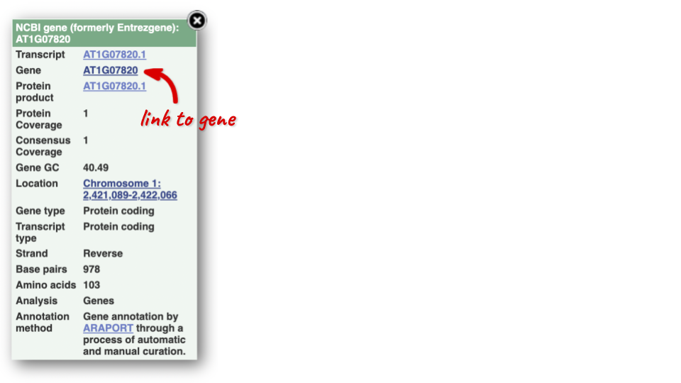
Alternatively, you can find a gene by searching for it. You can search for gene names or identifiers, and also phenotypes or functions that might be associated with the genes.
We’re going to look at the Arabidopsis thaliana PAI1 gene. From plants.ensembl.org, type PAI1 into the search bar and click the Go button.
The gene tab
Click on PAI1 from the search hits. The Gene tab should open:
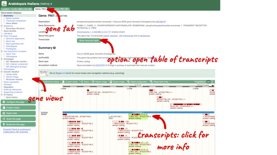
This page summarises the gene, including its location, name and equivalents in other databases. At the bottom of the page, a graphic shows a region view with the transcripts. We can see exons shown as blocks with introns as lines linking them together. Coding exons are filled, whereas non-coding exons are empty. We can also see the overlapping and neighbouring genes and other genomic features.
There are different tabs for different types of features, such as genes, transcripts or variants. These appear side-by-side across the blue bar, allowing you to jump back and forth between features of interest. Each tab has its own navigation column down the left hand side of the page, listing all the things you can see for this feature.
Let’s walk through this menu for the gene tab. How can we view the genomic sequence? Click Sequence at the left of the page.
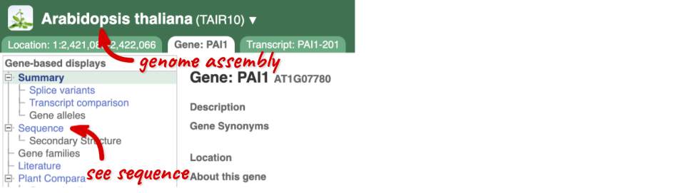
The sequence is shown in FASTA format. The FASTA header contains the genome assembly, chromosome, coordinates and strand (1 or -1) – this gene is on the negative strand.
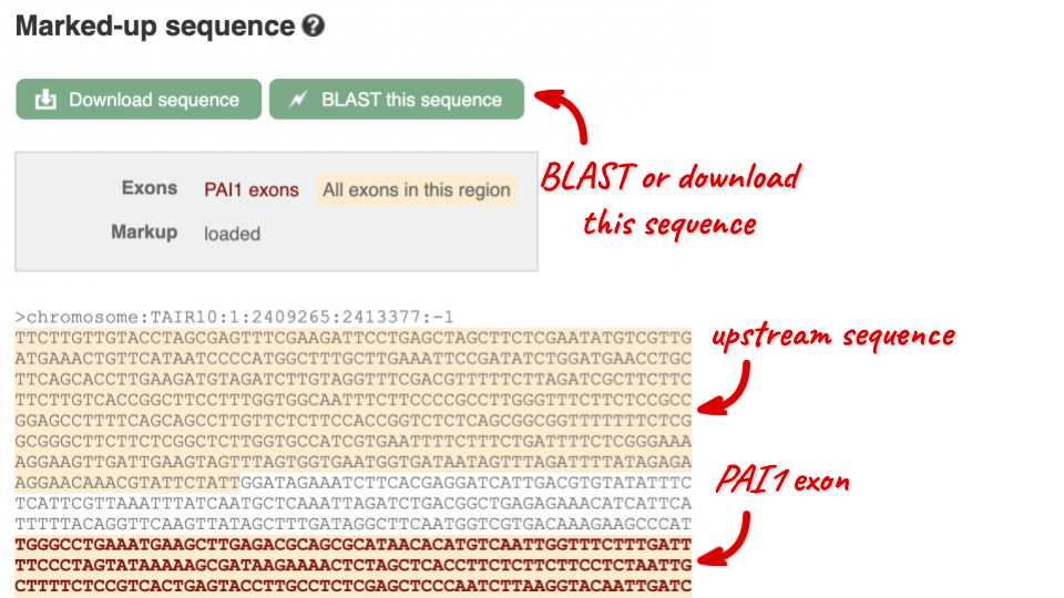
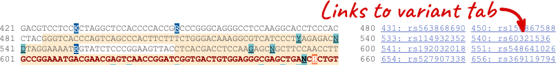
Exons are highlighted within the genomic sequence, both exons of our gene of interest and any neighbouring or overlapping gene. By default, 600 bases are shown up and downstream of the gene. We can make changes to how this sequence appears with the blue Configure this page button found at the left. This allows us to change the flanking regions, add variants, add line numbering and more. Click on it now.

Once you have selected changes (in this example, Show variants and Line numbering) click at the top right.
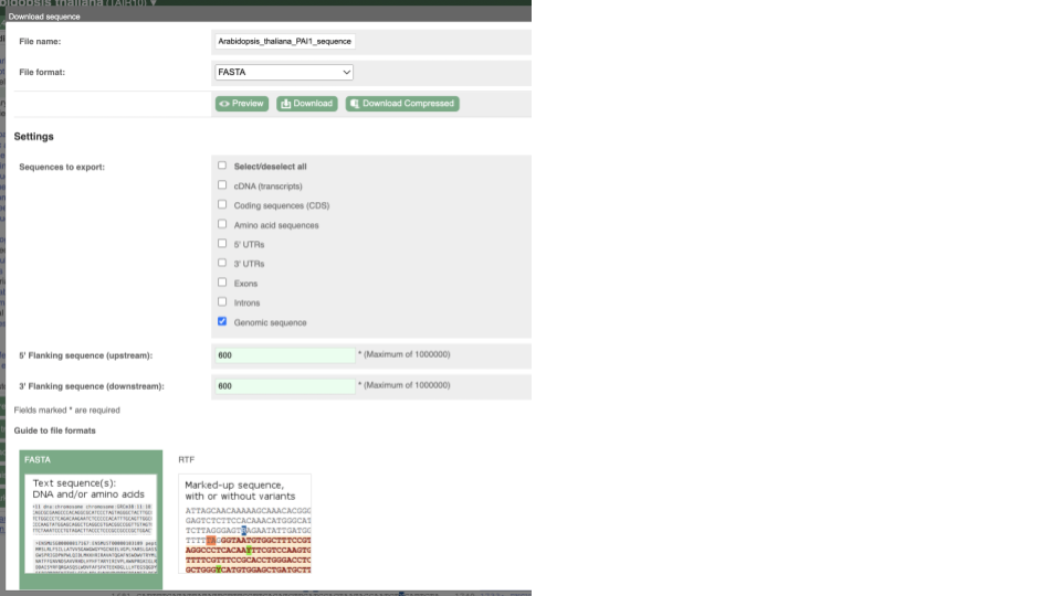
You can download this sequence by clicking in the Download sequence button above the sequence:
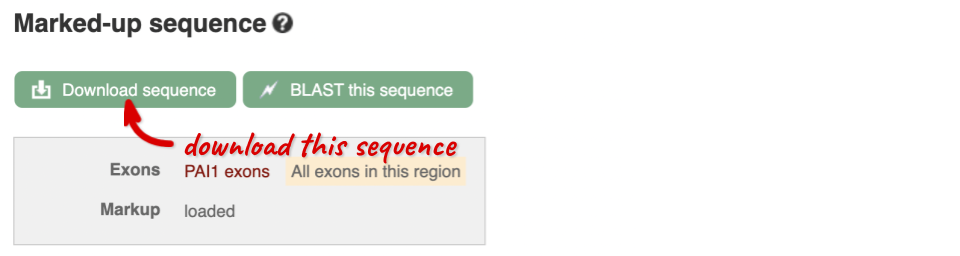
This will open a dialogue box that allows you to pick between plain FASTA sequence, or sequence in RTF, which includes all the coloured annotations and can be opened in a word processor. If you want run a sequence analysis tool, download as FASTA sequence, whereas if you want to analyse the sequence visually, RTF is best for this. This button is available for all sequence views.
To find out what the protein does, have a look at GO terms from the Gene Ontology consortium. There are three pages of GO terms, representing the three divisions in GO: Biological process (what the protein does), Cellular component (where the protein is) and Molecular function (how it does it). Click on GO: Biological process to see an example of the GO pages.
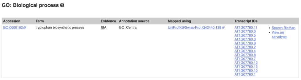
Here you can see the functions that have been associated with the gene. There are three-letter codes that indicate how the association was made, as well as links to the specific transcript they are linked to.
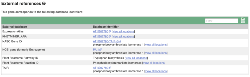
We also have links out to other databases which have information about our genes and may focus on other topics that we don’t cover, like Expression Atlas or UniProtKB. Go up the left-hand menu to External references:
Demo: The transcript tab
We’re now going to explore the different transcripts of PAI1. Click on Show transcript table at the top.
![]()
![]()
Here we can see a list of all the transcripts of PAI1 with their identifiers, lengths and biotypes. Click on the ID of the Ensembl Canonical transcript, PAI1-211.
You are now in the Transcript tab for PAI1-211. We can still see the gene tab so we can easily jump back. The left hand navigation column provides several options for the transcript PAI1-211 - many of these are similar to the options you see in the gene tab, but not all of them. If you can’t find the thing you’re looking for, often the solution is to switch tabs.
Click on the Exons link. This page is useful for designing RT-PCR primers because you can see the sequences of the different exons and their lengths.
![]()
You may want to change the display (for example, to show more flanking sequence, or to show full introns). In order to do so click on Configure this page and change the display options accordingly.
Now click on the cDNA link to see the spliced transcript sequence with the amino acid sequence. This page is useful for mapping between the RNA and protein sequences, particularly genetic variants.
![]()
UnTranslated Regions (UTRs) are highlighted in dark yellow, codons are highlighted in light yellow, and exon sequence is shown in black or blue letters to show exon divides. Sequence variants are represented by highlighted nucleotides and clickable IUPAC codes are above the sequence.
Next, follow the General identifiers link at the left. Just like the External References page in the gene tab, this page shows links out to other databases such as RefSeq, UniProtKB, PDBe and others, this time linked to the transcript or protein product, rather than the gene.
![]()
If you’re interested in protein domains, you could click on Protein summary to view domains from Pfam, PROSITE, Superfamily, InterPro, and more. These are all plotted against the transcript sequence, with the exons shown in alternating shades of purple at the top of the page. Alternatively, you can go to Domains & features to see a table of the same information.
![]()
![]()
Comparative genomics
Demo: Exploring comparative genomics data for cultivars in Ensembl Plants
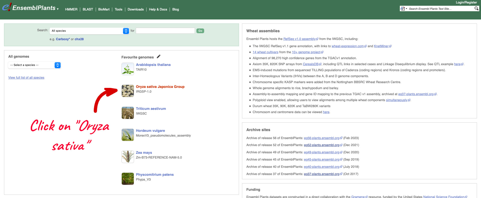
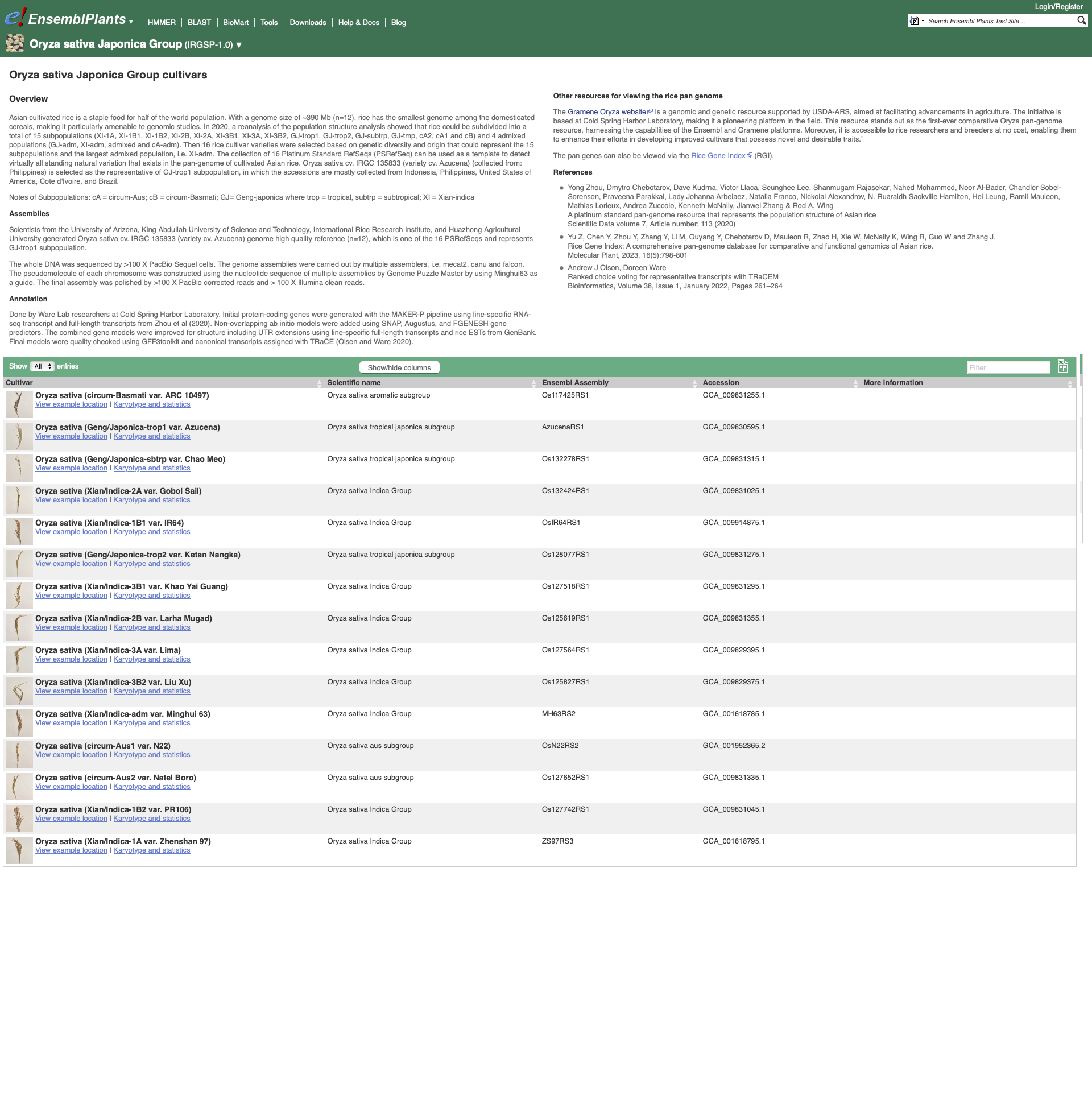
To see the list of cultivars available for your chosen species, select the reference genome for that species. We are going to select Oryza sativa Japonica Group which will take you to the genome’s home page:
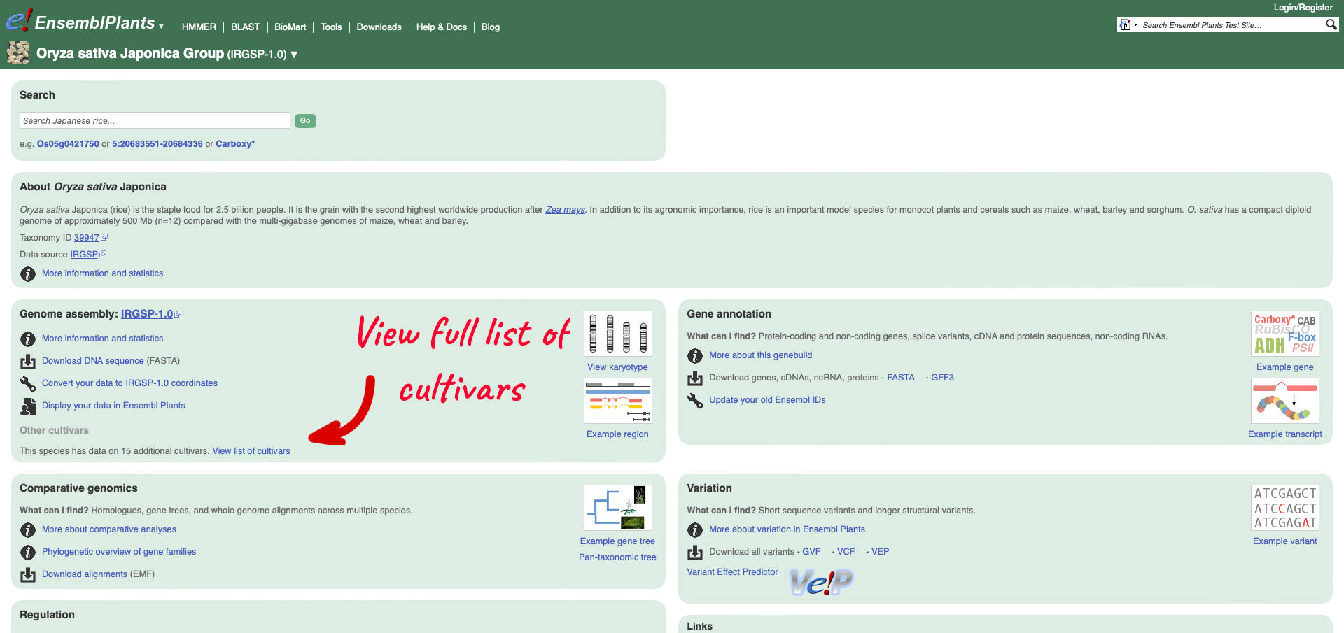
Within the Genome Assembly area there will be a link to ‘View full list of cultivars’ when additional cultivars are available in Ensembl. Clicking this link will take you to a list of all available cultivars, with some overview information and links to access example locations or the genome’s home page for each cultivar.
Returning to the Ensembl Plants homepage, we can search for rice gene Os05g0421300.
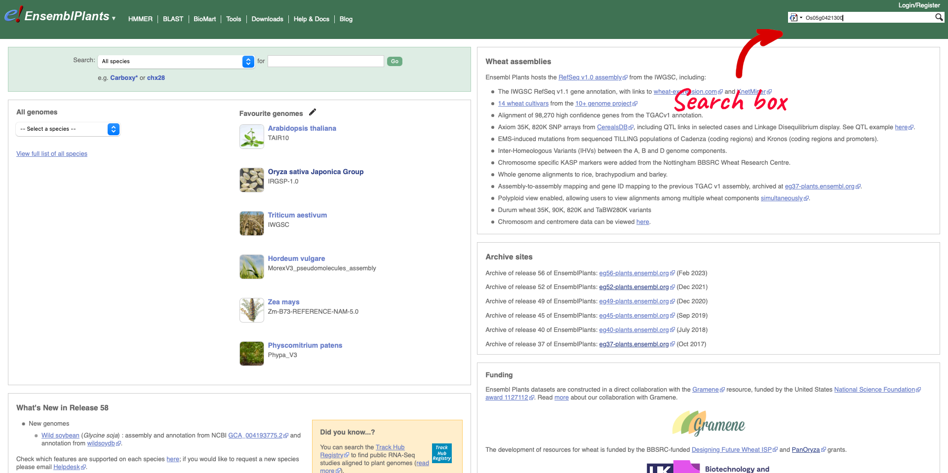
The results return links to the gene page, species home page, location (Chromosome 5: 20,663,027-20,668,604) and gene tree. We are going to select the Gene from species “Oryza sativa Japonica Group”.
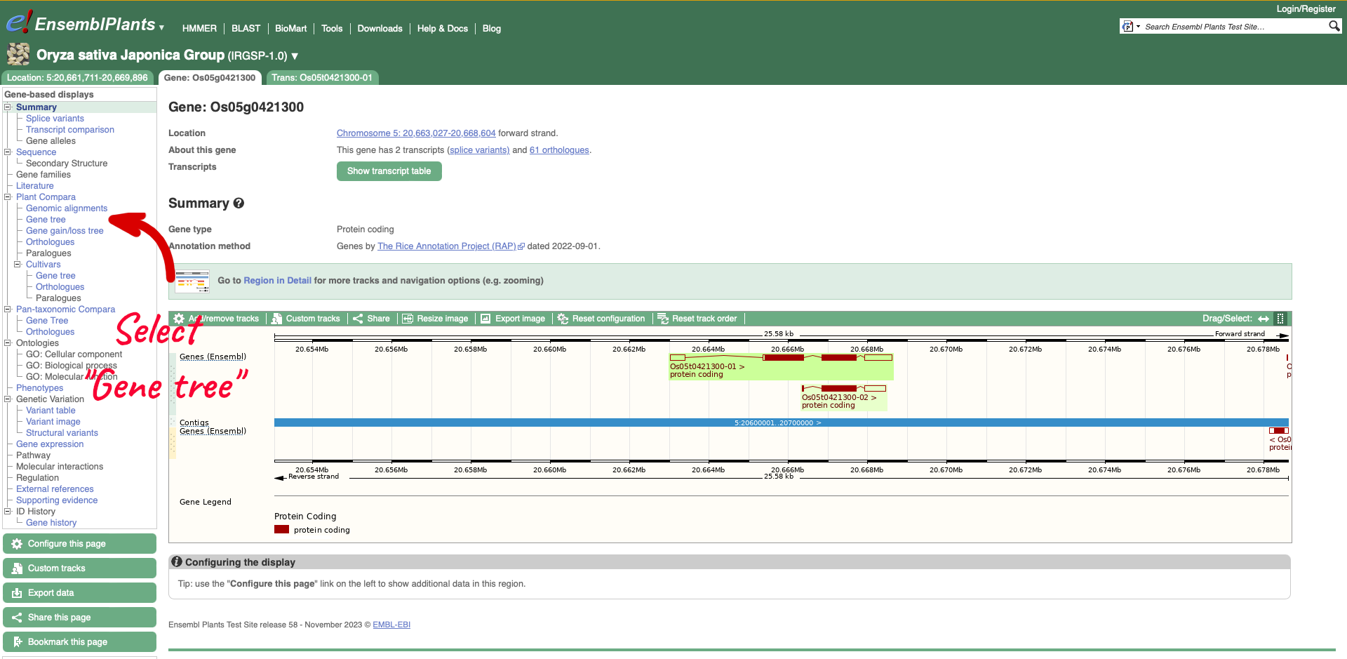
On the left-hand menu there is a sub-menu called ‘Plant Compara’ and a menu within that for ‘Cultivars’. We will select ‘Gene tree’ which will show a gene tree generated by the Gene Orthology/Paralogy prediction method pipeline. Cultivar gene trees are constructed using one representative protein (typically the longest protein-coding translation) for every gene in each cultivar. Cultivars whose genomes have been assembled into chromosomes and have been independently annotated are included into Cultivar comparative analyses.
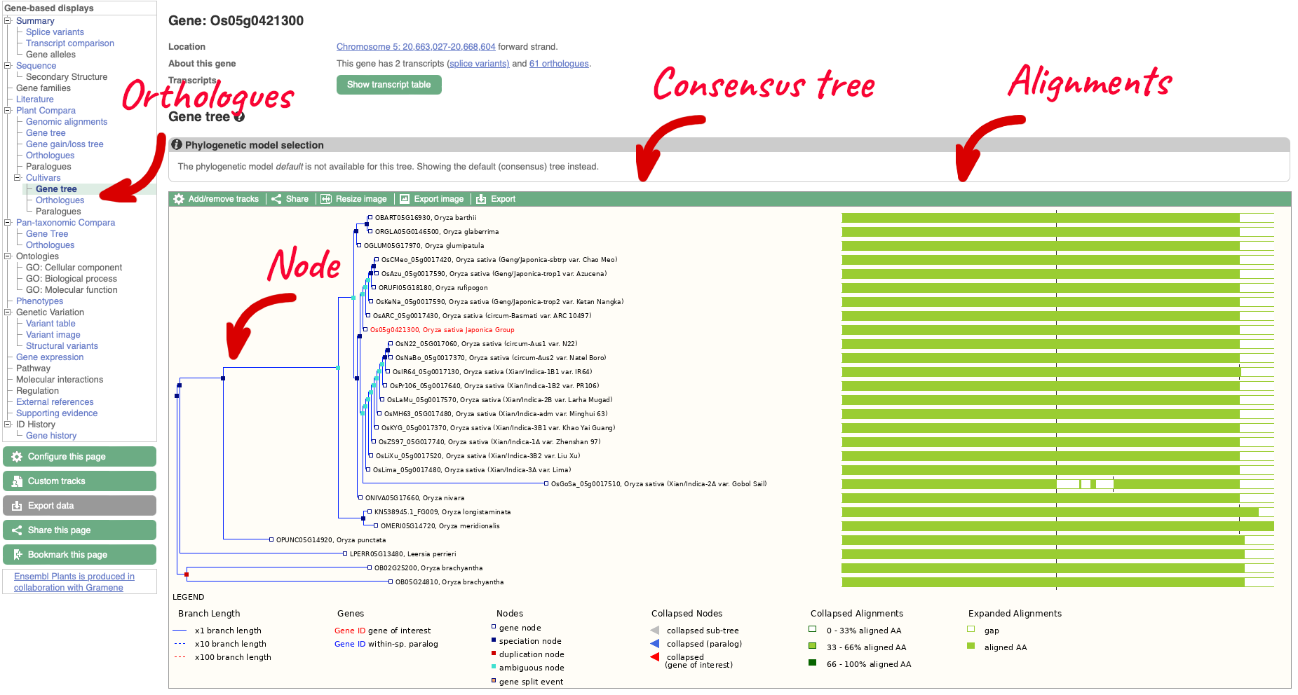
The display shows the consensus tree representing the evolutionary history of this gene and an image of the alignments. Subtrees can be expanded by clicking on a node (blue or red squares) and selecting ‘expand this subtree’ from the pop-up menu. The gene of interest is displayed with red text.
For this example we can see that the two ‘circum-Aus’ cultivars cluster with the ‘Xian/indica’ cultivars, and that the ‘circum-Basmati’ clusters with the ‘Geng/Japonica’ cultivars. Additional Oryza wild relatives are also shown, along with outgroup Leersi perrieri. We can also see from the alignments that the gene is highly conserved, but the representative protein in cultivar ‘Gobol Sail’ has some gaps compared to the others.
On the left-hand menu we can select ‘Orthologues’ from the Cultivar sub-menu of the ‘Plants compara’ menu. This will bring up a table of orthologues which have been inferred from the gene tree. The table lists the species, type of orthologue (e.g. 1-to-1, 1-to-many), links to jump to an orthologue’s gene page, region comparison page (to see an alignment image of the two genes) or text cDNA/protein alignments. Information detailing the percentage identity of the query and target sequences, Gene order conservation (GOC) score, whole genome alignment (WGA) coverage and indication of high confidence (Yes for homology with high percentage identity and high GOC or WGA coverage) are also provided.
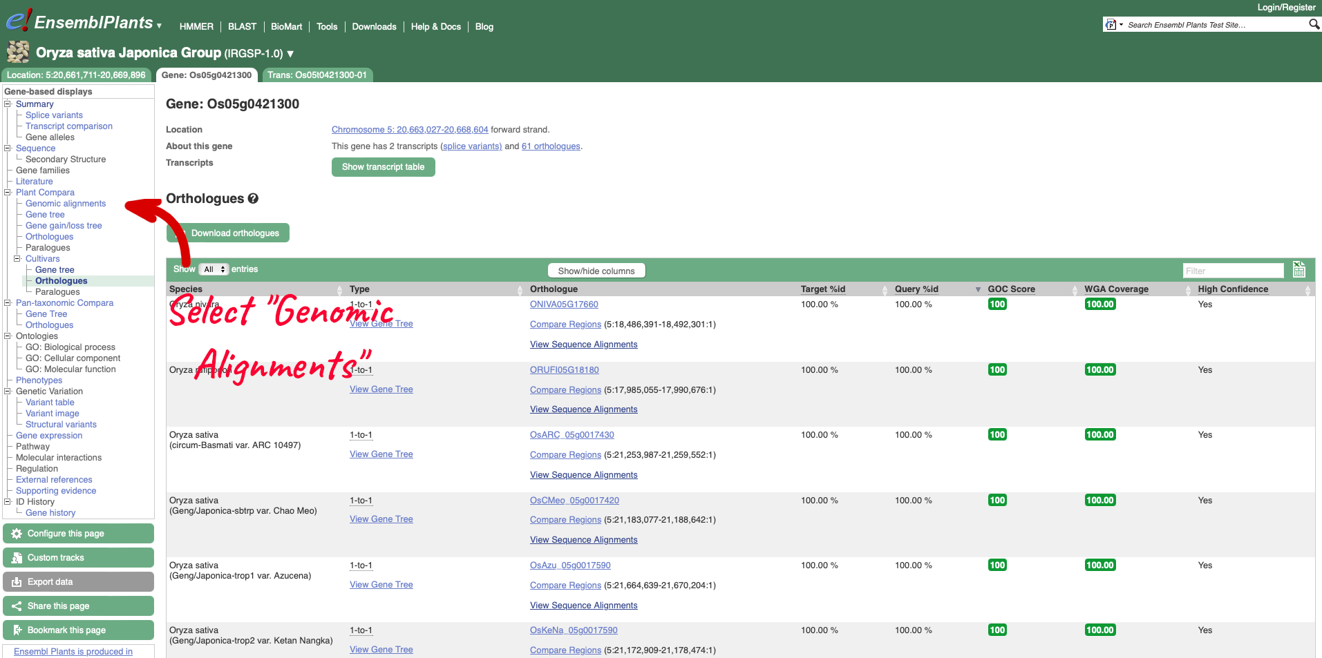
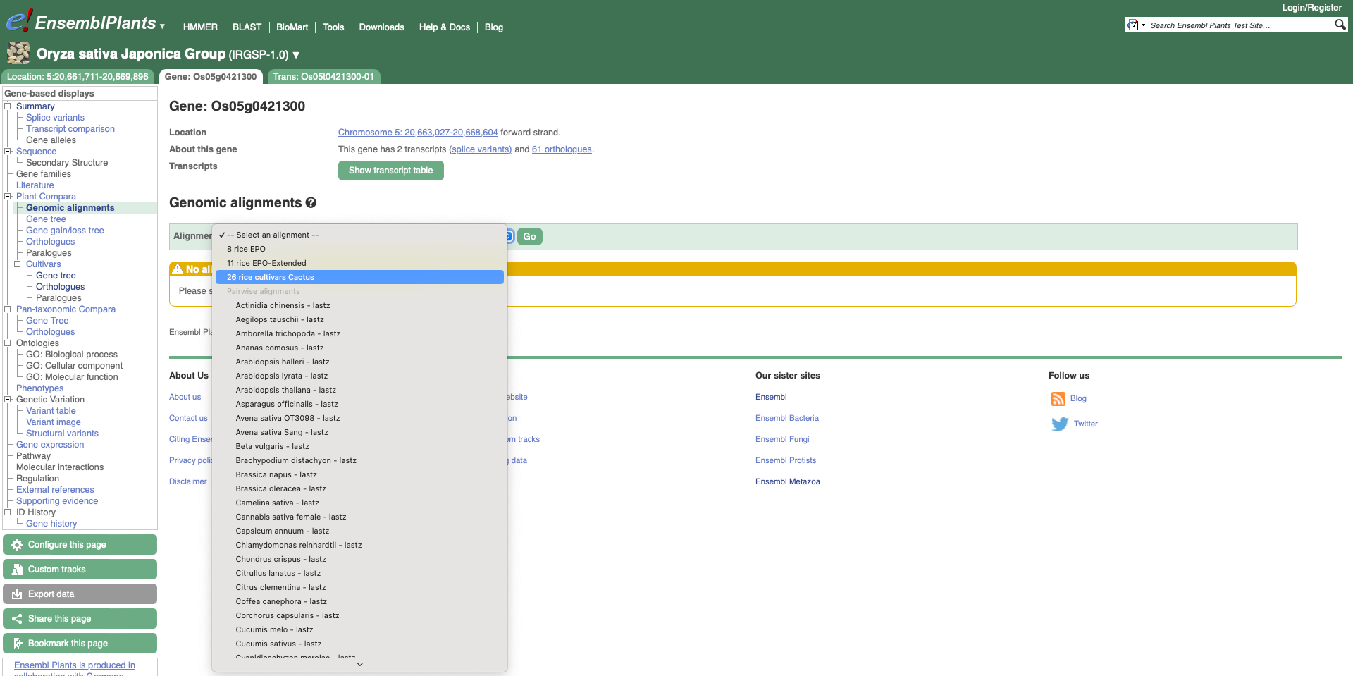
To visualise whole genome alignments in this region, we can use the left-hand menu to select ‘Genomic Alignments’ from the ‘Plants compara’ sub-menu. We can then select which alignment we want to display. Options include multiple genome alignments using the EPO (Enredo, Pecan, Ortheus) pipeline or progressive cactus for cultivar alignments. Pairwise alignments generated with LASTZ or cactus are also available for comparison to other plant species, or other cultivars. We will select the ’26 rice cultivars cactus’ alignment to display.
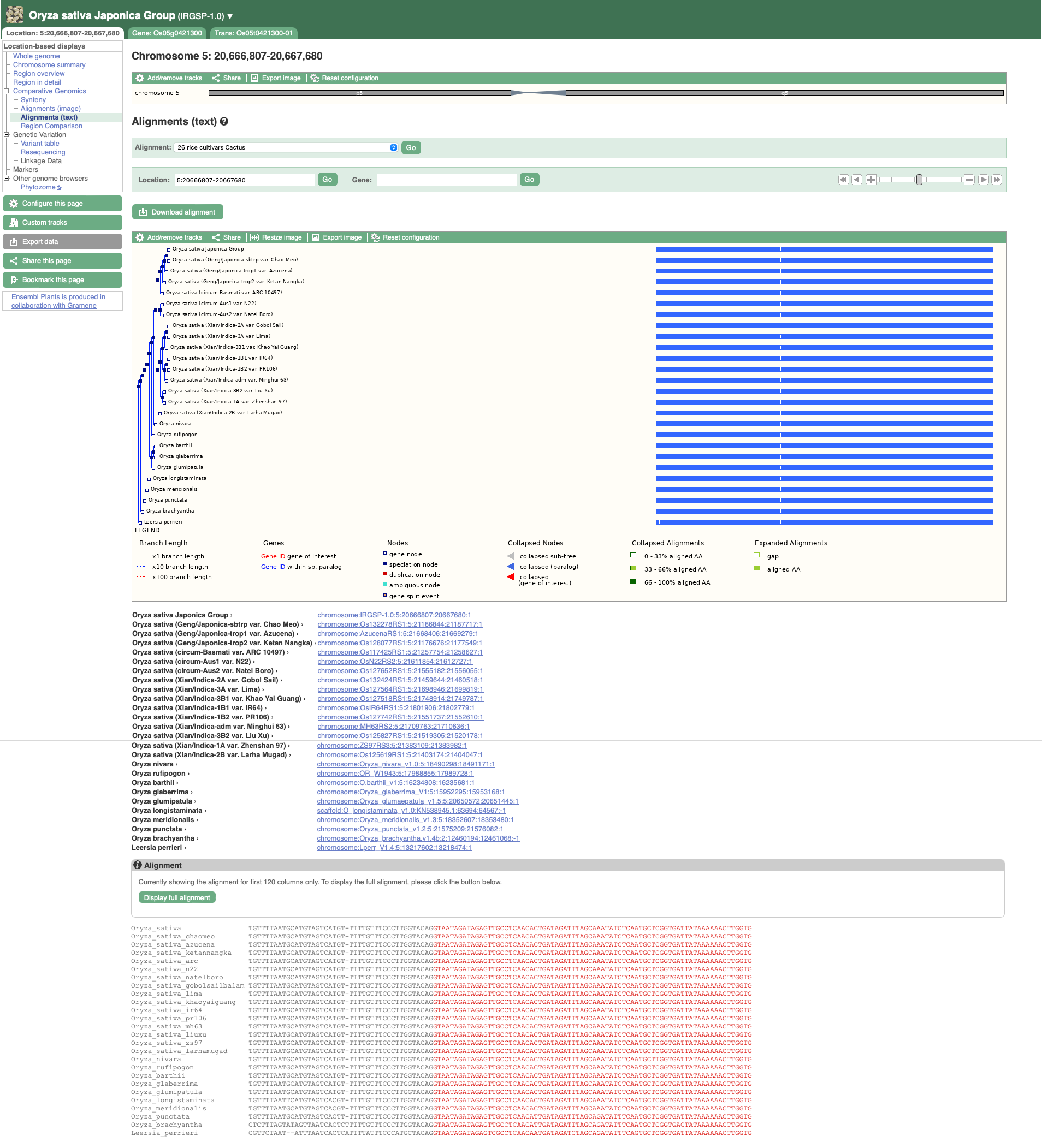
The resulting alignment is returned in a series of blocks, arranged from longest (block 1) to shortest. The table can also be sorted by location on the reference genome. To view a block’s alignment, click on the name of the block. A tree view depicts the tree from cactus, with the sequence alignment represented on the right. Below the tree view a list of links to each aligned region is provided, and below that the text representation of the alignment with exons shown in red.
Ensembl Rapid Release
Newly imported genomes are added to Ensembl Rapid Release. These genomes have minimal annotation, with genes mapped onto the genome, InterProScan protein domain analysis and BLAST indexing. Lightweight homology predictions are provided rather than full comparative genomics analysis, and there is no BioMart.
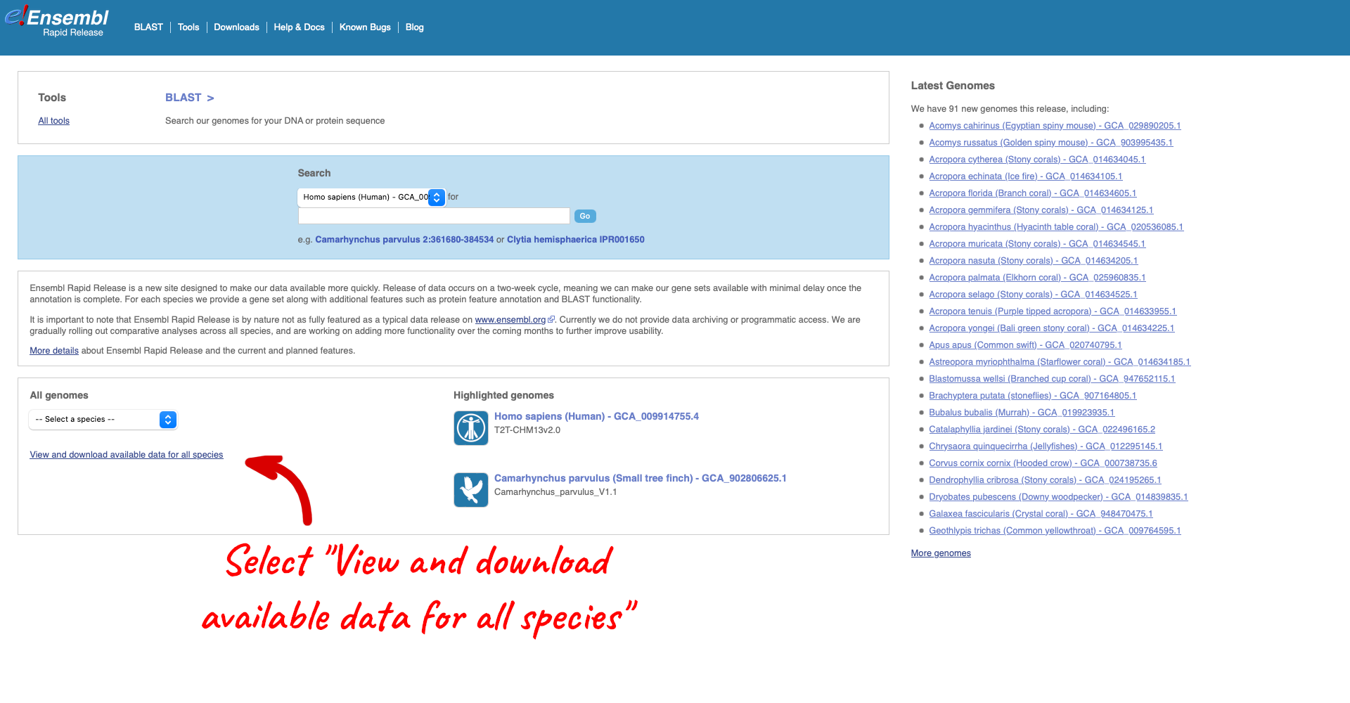
From the Rapid Release homepage, click on View and download available data for all species.
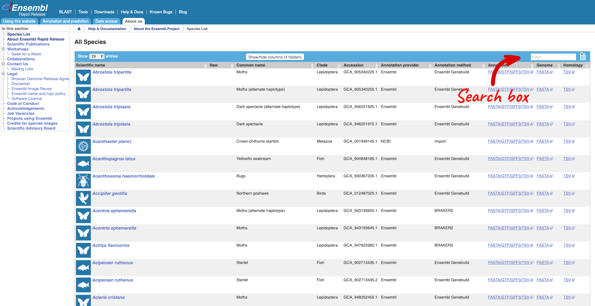
Here we have a list of all the species available in Rapid Release, including latin and common names, genome accession and annotation source. There are also links out to the FTP site where you can download whole genome flatfiles.
Use the search box to search for “Diabrotica balteata” which is the scientific name for the Cucumber beetle.
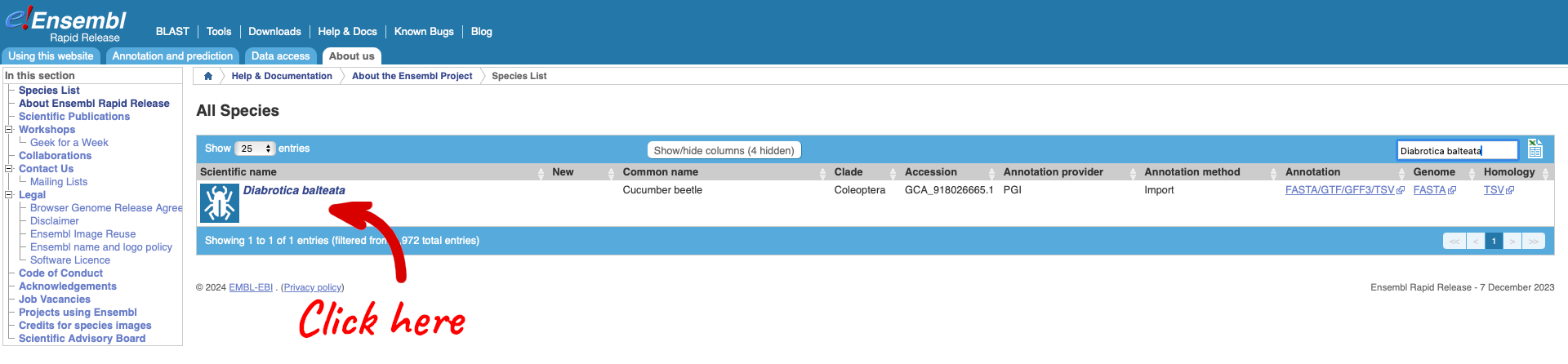
Clicking on the scientific name will take you to the species page. Here you can see links to example data and statistics about the genome. Clicking on the example gene “DIABBA_LOCUS6468” will take you to its gene page.
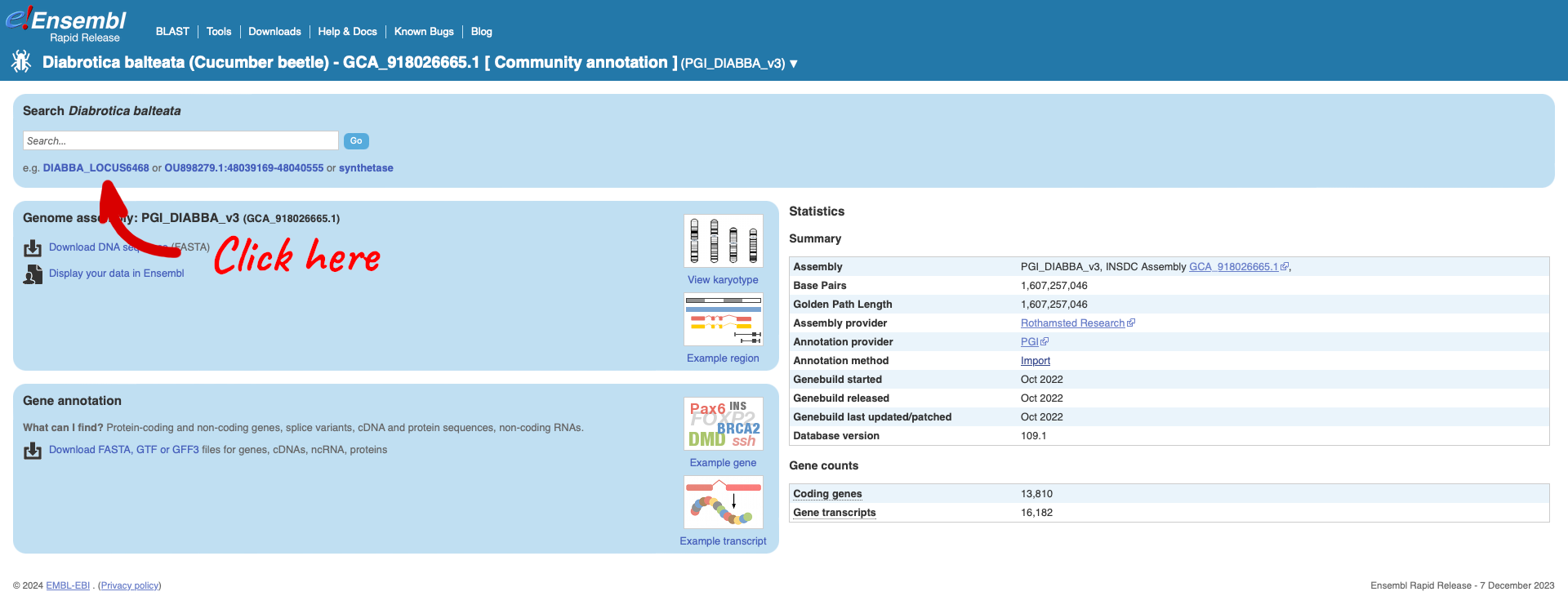
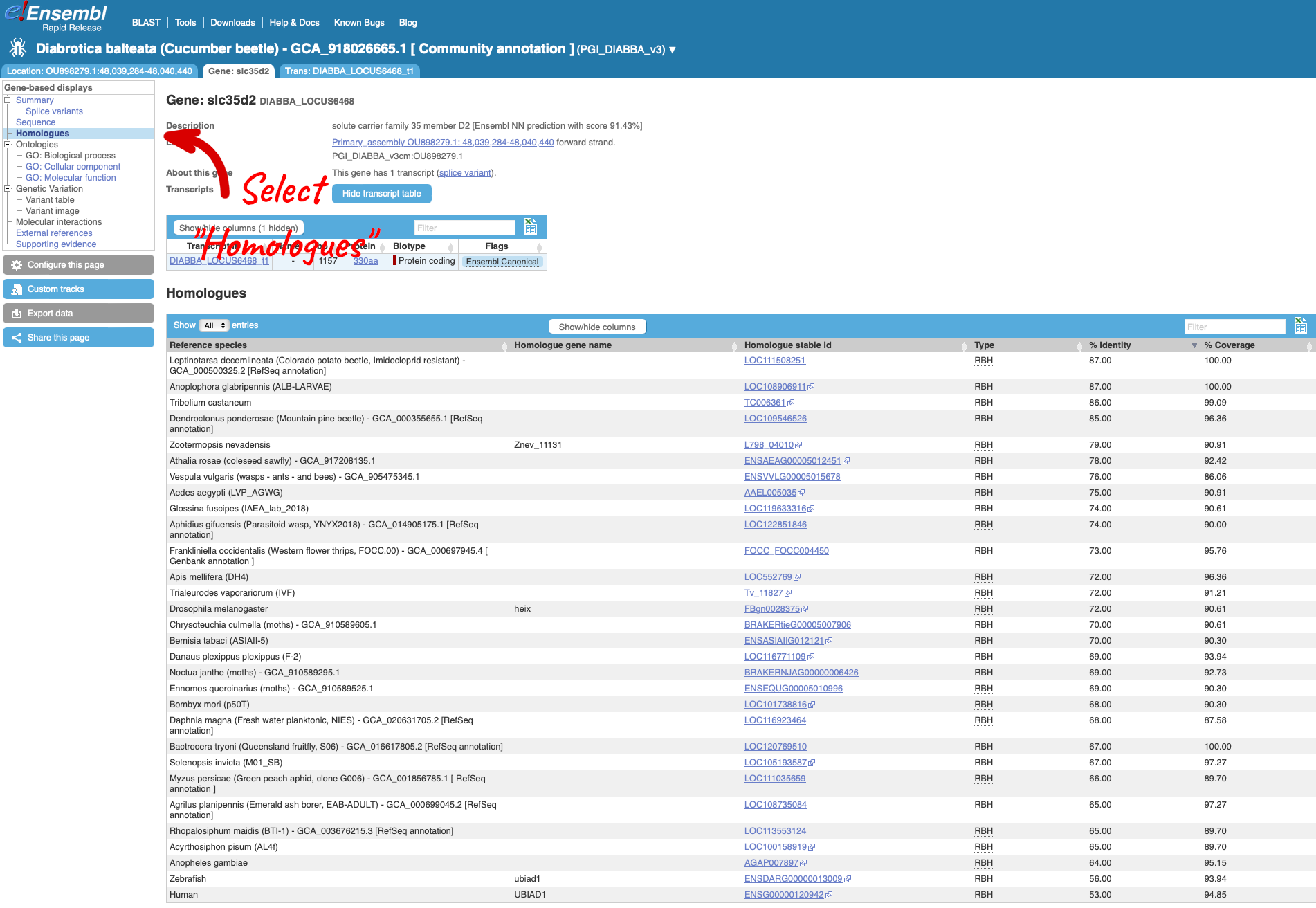
The gene page has a summary of the gene information, including a table of the transcripts. Selecting ‘Homologues’ from the left-hand menu will load a table showing a list of homologues calculated between the cucumber beetle slc35d2 gene and a set of genome representatives primarily from insect species.
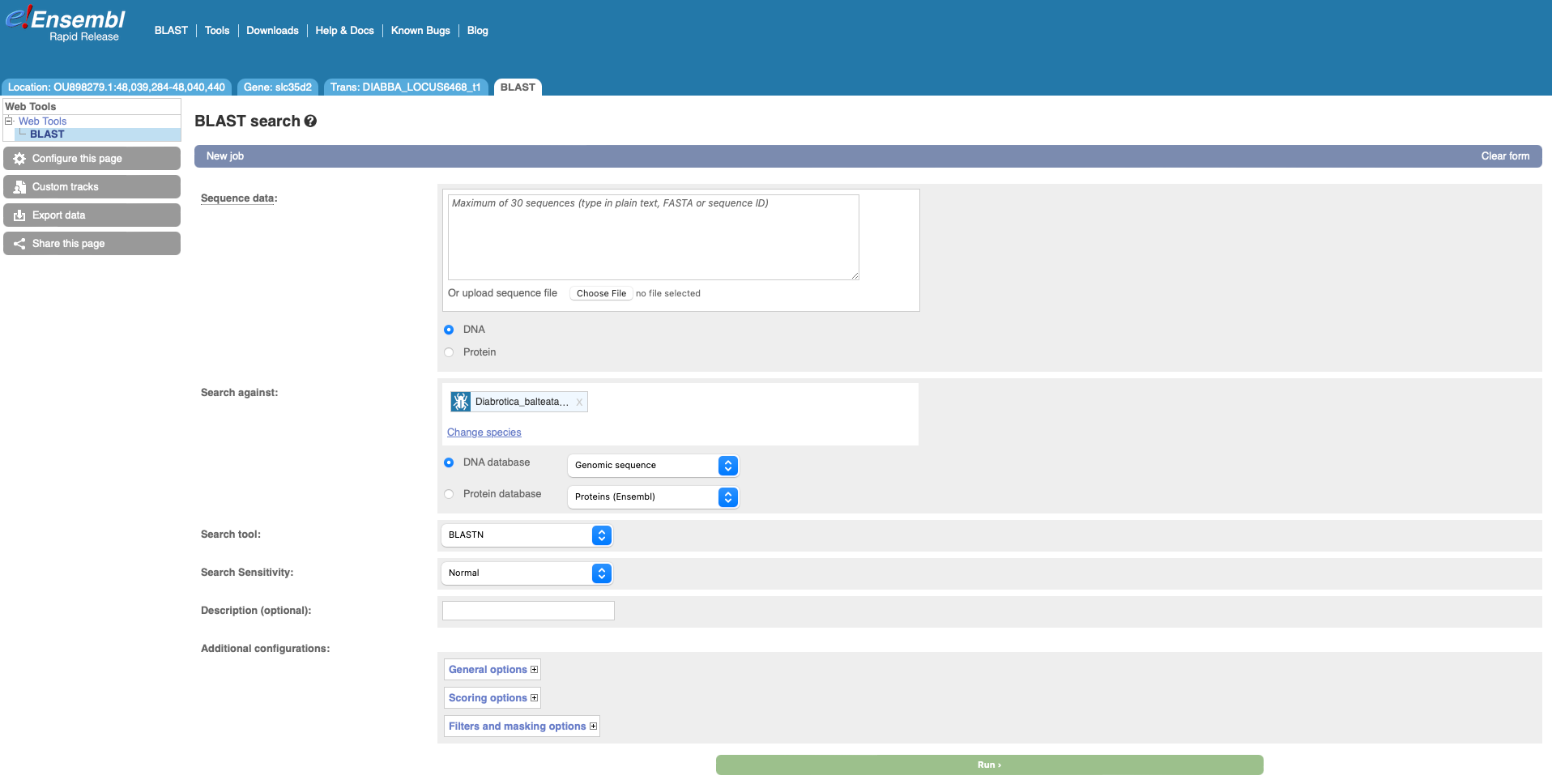
Rapid also has BLAST functionality – you can find the link to the BLAST tool located in the tool bar at the top of the screen. Following the link to use the BLAST tool, you will see that the cucumber beetle has automatically been selected as the target genome. You can now run BLAST searches for DNA or protein sequences.
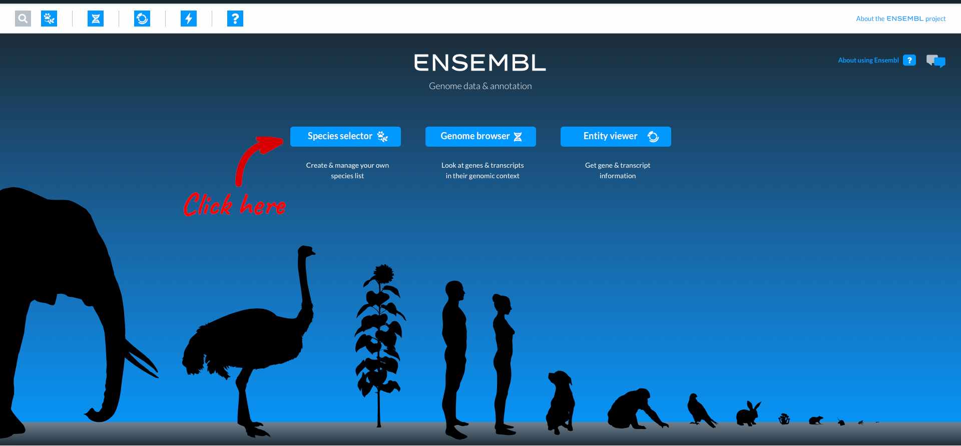
Ensembl Beta
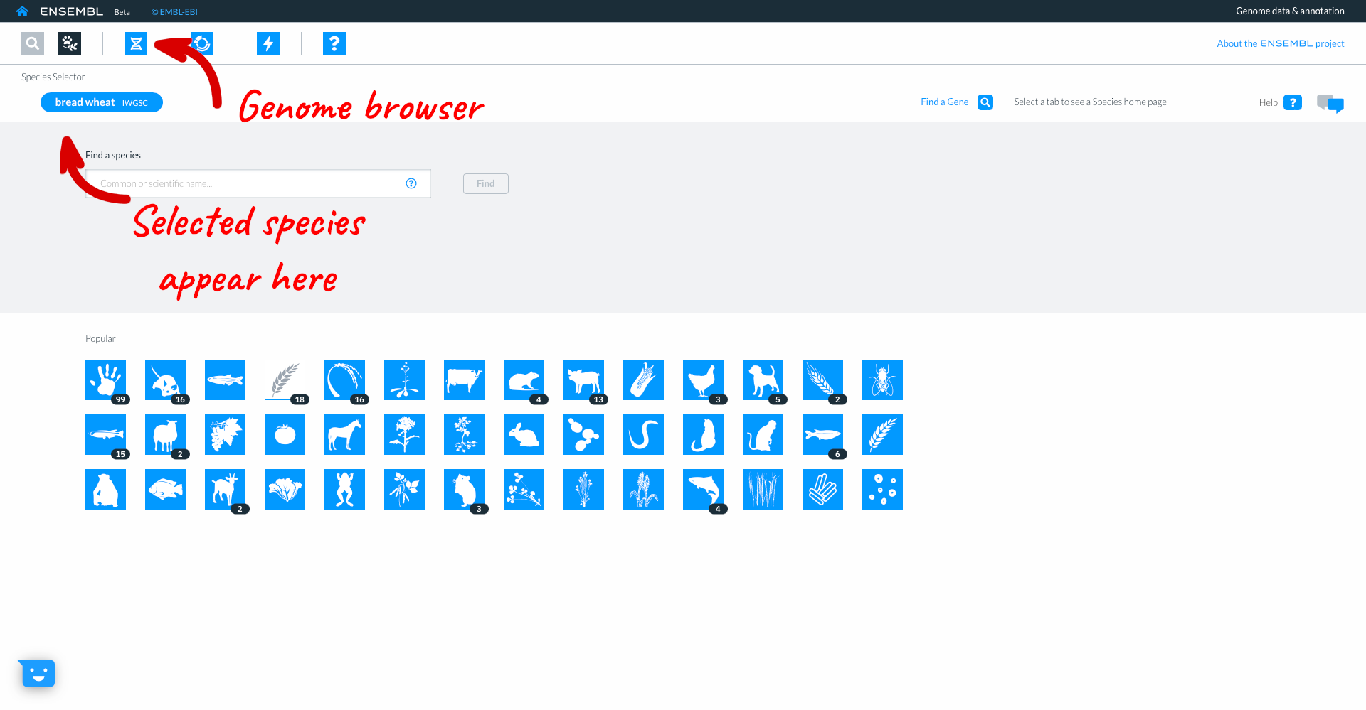
This is the homepage for the new Ensembl, which is currently released as a beta version. Over time additional species and functionality will be added, but for now let’s start by choosing a species using the “Species selector”.
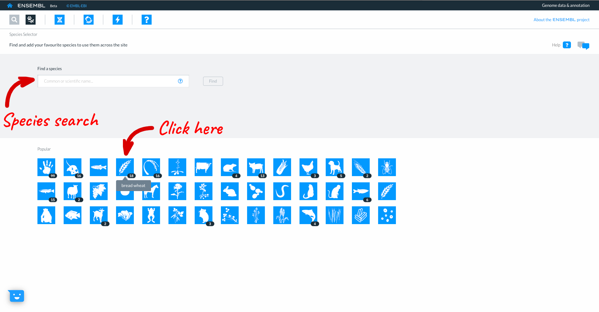
Here you can see icons for the most popular species in Ensembl, comprising vertebrates, invertebrates, plants, fungi and microbes. You can select a species to work with by clicking on the icon. The numbers in black lozenges at the bottom corner of species icons show where we hold more than one assembly for that species. You can also select species by typing into the species search box. We are going to work with wheat, so click on the wheat icon.
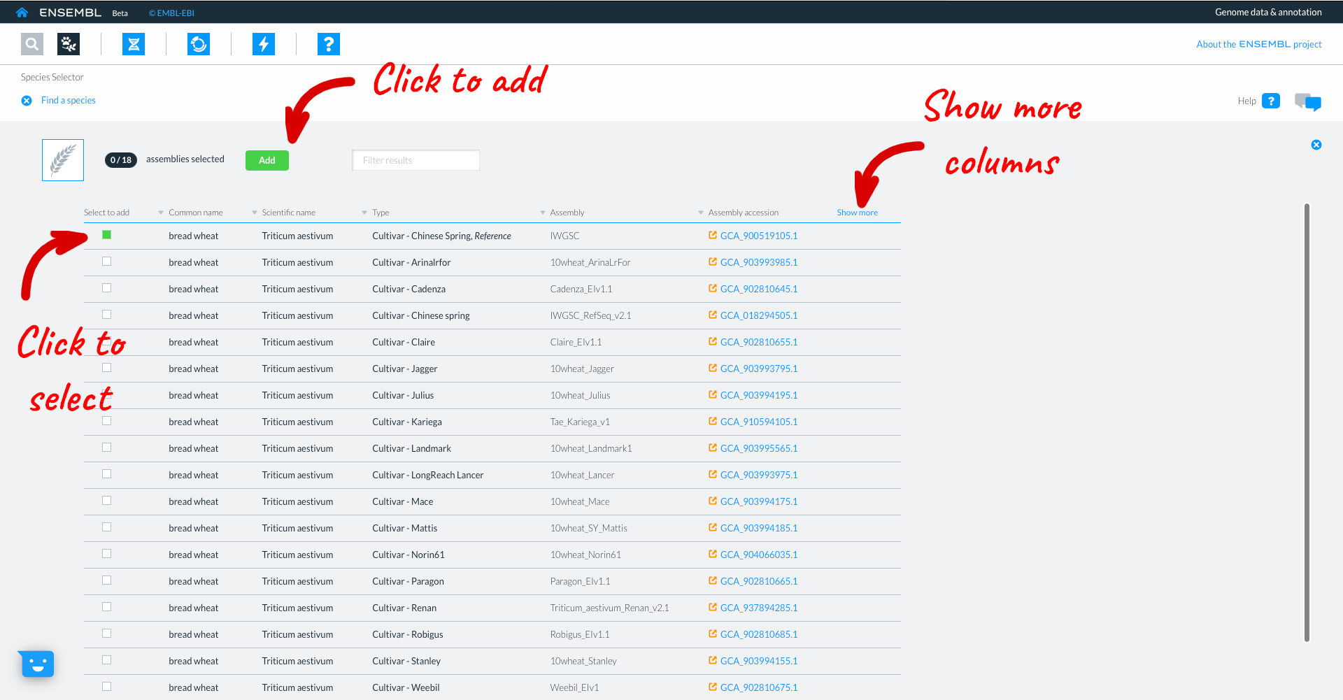
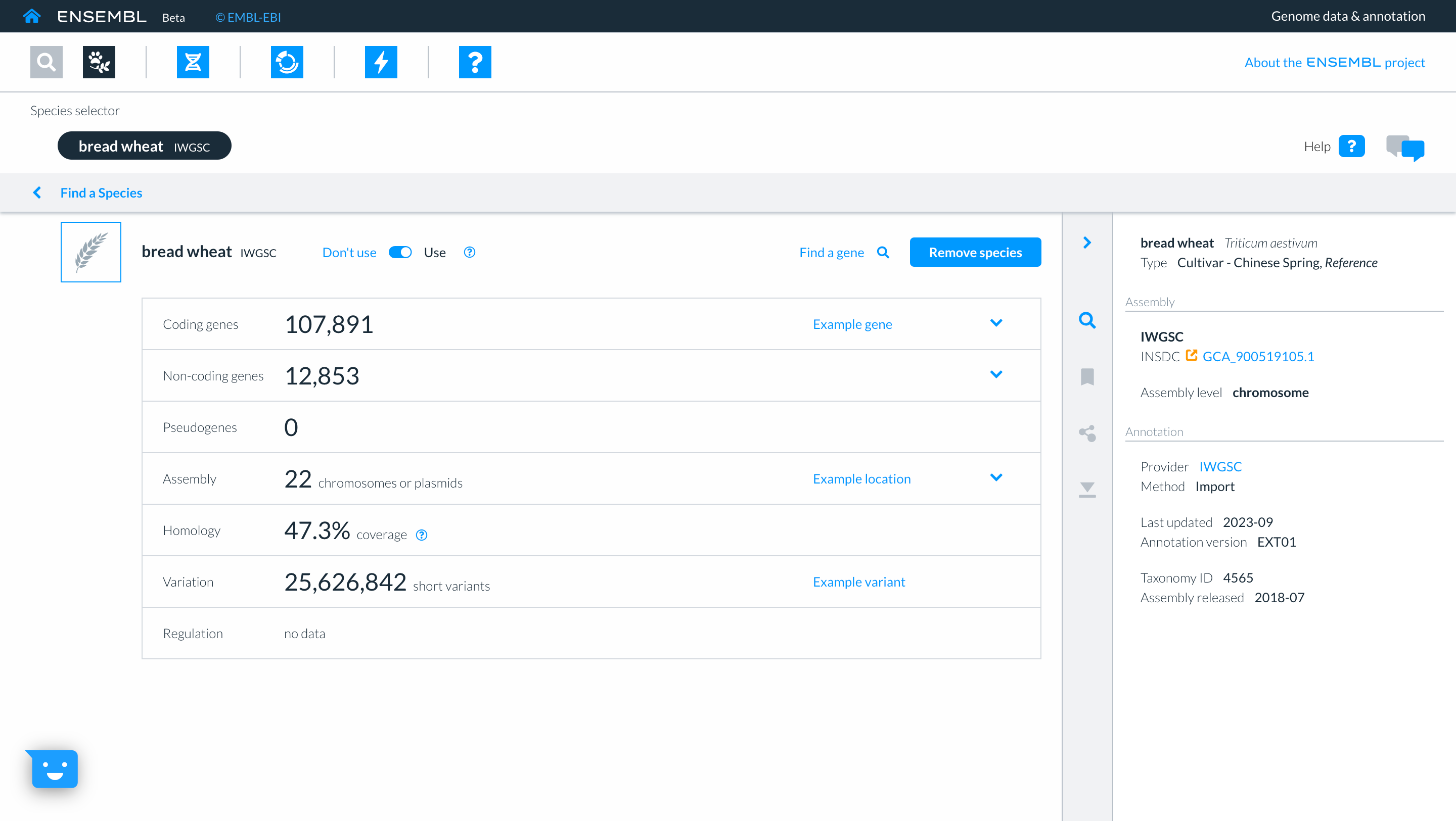
This takes you to the list of available wheat genomes currently available in Beta Ensembl. The table provides information such as common name, scientific name, and information about the assembly. Clicking ‘show more’ reveals additional columns with information relating to the assembly quality and additional data types associated with that assembly. You can select genomes to work with by clicking the square button to the left of each genome. We will select the wheat reference IWGSC assembly, then click “Add”.
Clicking on the genome name in the top panel will take you to the species page for that genome where more detailed information and statistics relating to that assembly are displayed.
Returning to the species selector by clicking on ‘Find a species’, you can now see the genomes which you have selected in the upper part of the screen. Here too you have icons to access other parts of Ensembl. For now we will click on the ‘Genome Browser’ icon and then searching for gene “TraesCS3D02G273600”.
The genome browser shows gene model TraesCS3D02G273600 with exons in blue boxes, introns as lines and UTR as open boxes. The wiggle plot shows the GC content, while the bottom track show variants coloured by consequence. The right hand panel gives more information about the transcripts in the focus gene.
![]()
If you click on the transcript model a pop-up appears with an overview of the gene and Download options for the different sequences e.g. genomic, cDNA, protein or CDS. ![]()
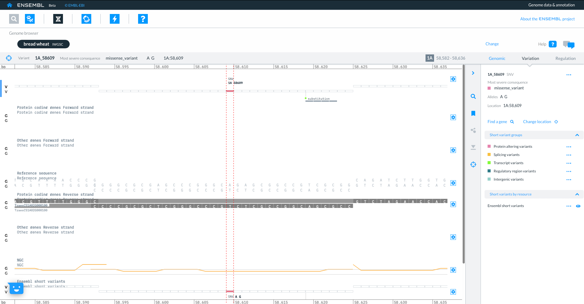
If you zoom in you can focus on the individual variants, with further details shown in the right hand panel
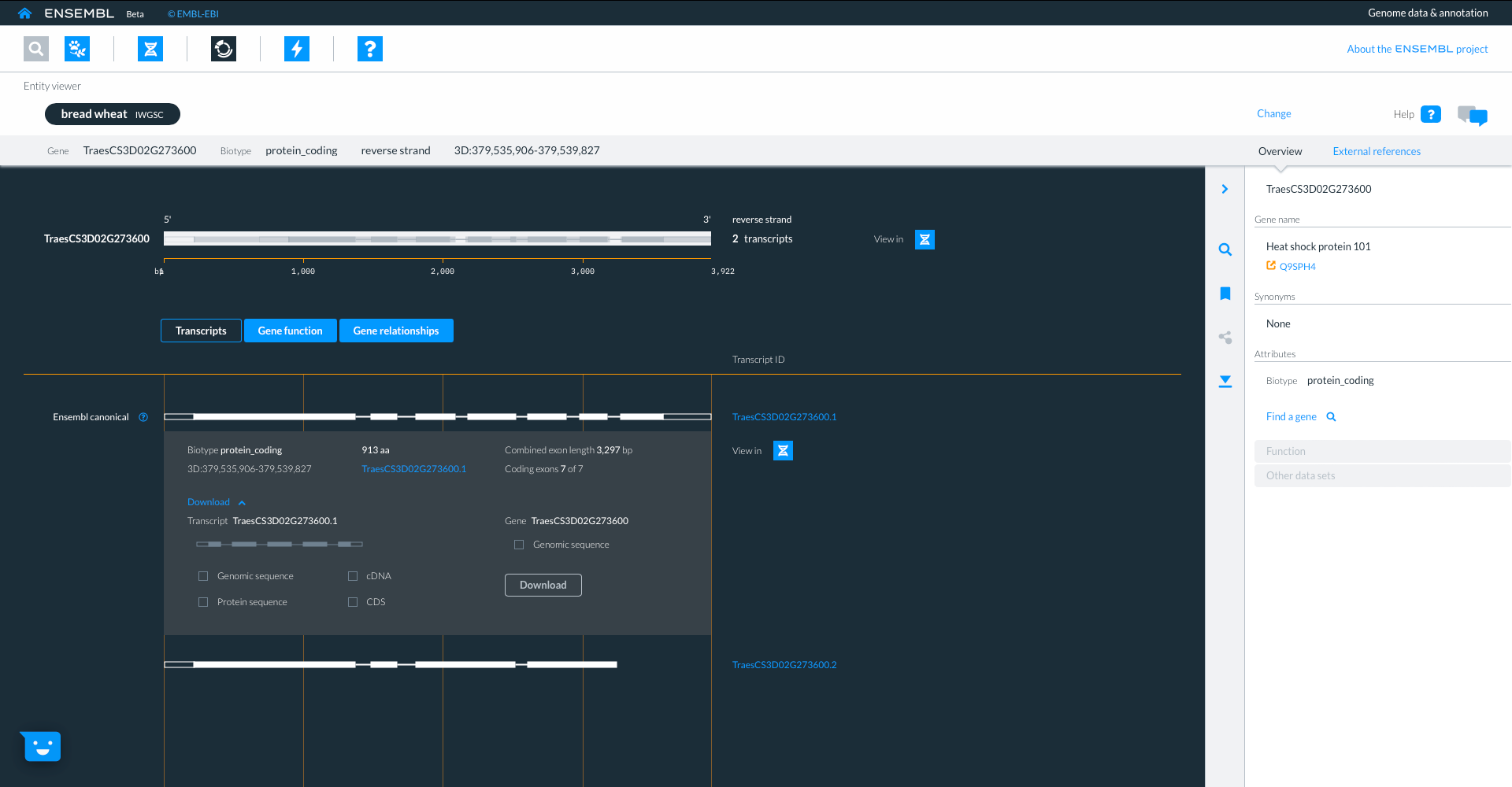
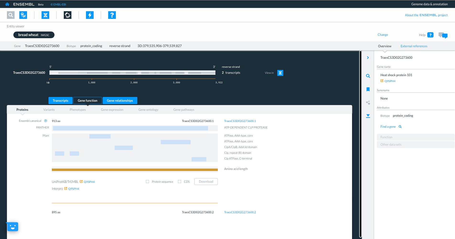
Using the icons in the top panel we can also go to the entity viewer, where we can find more details about the entities in question. Here we are focused on the same gene TraesCS3D02G273600 and we can view and download sequence from the individual transcripts.
We can also look at the ‘Gene function’ tab where we see information about protein domains, with links to Uniprot and Interpro. We can also see information on variants, phenotypes, gene expression and pathway information where available.
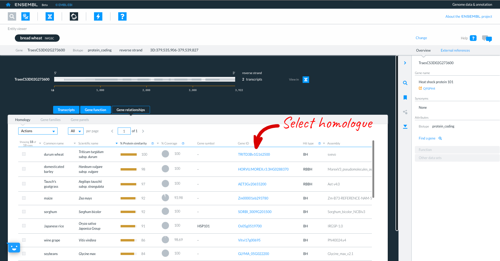
Selecting the third tab “Gene relationships” shows homology information to other ensembl species, with details about sequence similarity and how the hit was identified. By selecting links to homologue gene IDs we can jump to the homologues gene in another species. We will select gene “TRITD3Bv1G162500” from Triticum turgidum ssp. Durum.
Here we see the Durum gene, in the entity viewer. The focus species is coloured in black, but the original species (in our case Bread wheat T. aestivum remains listed to allow for easy switching between the two).
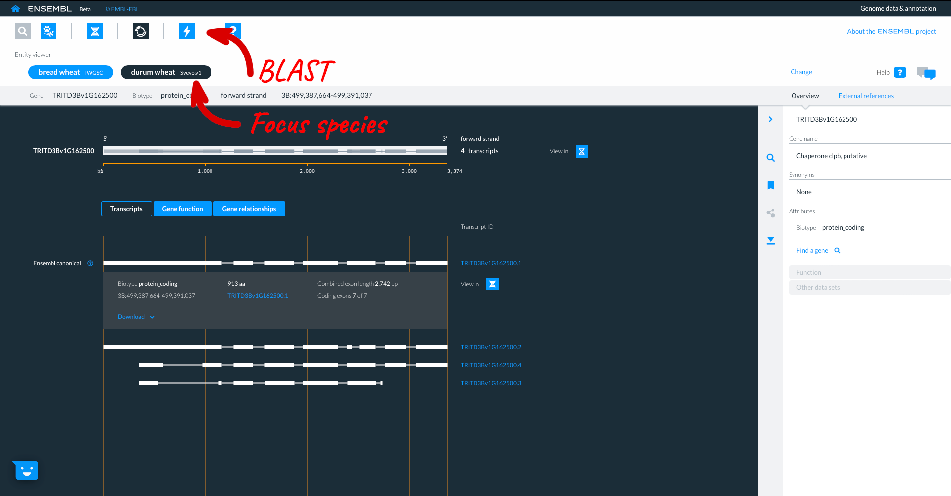
Beta Ensembl has BLAST functionality which can be accessed by clicking on the lightning icon in the top panel. Where you can currently BLAST up to 50 sequences against up to 25 species.
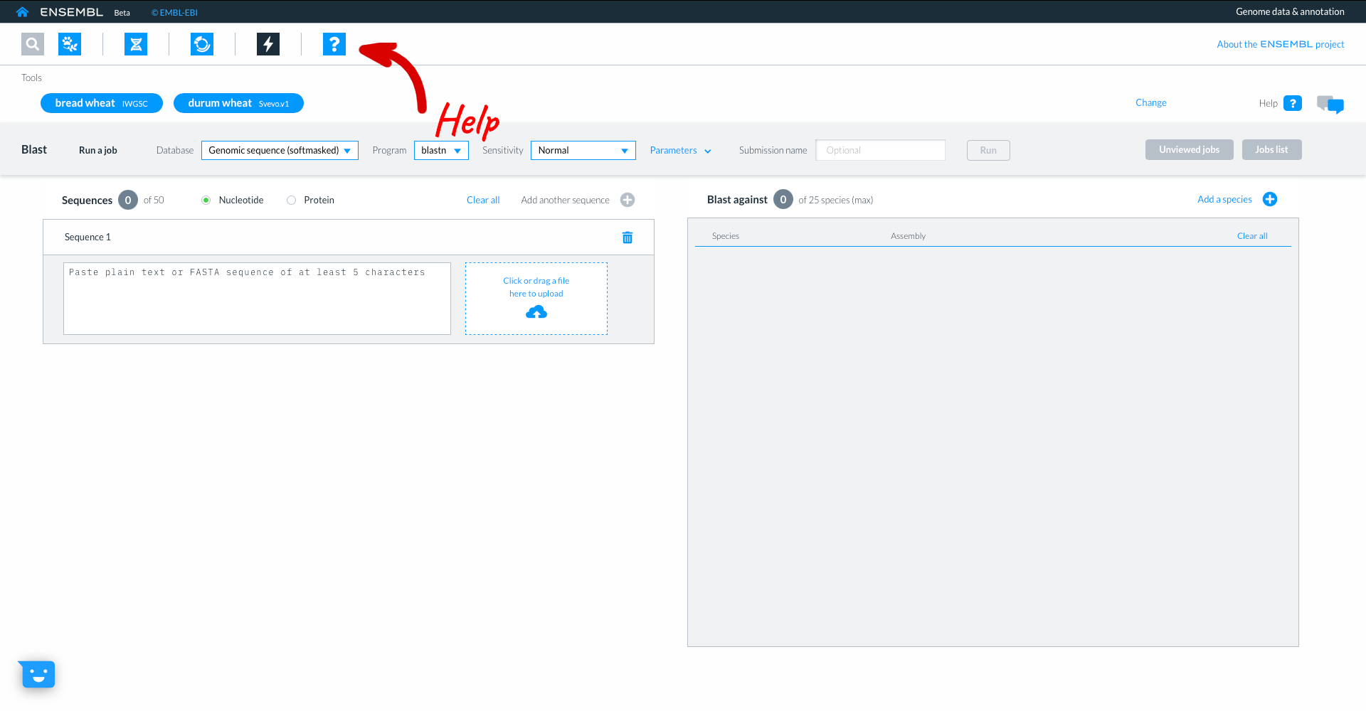
The final icon with the ‘?’ links to our help and documentation where you can learn more about the different Ensembl apps.
On every page you will also find a speech bubble icon where you can quickly feedback on your experience when using the site.
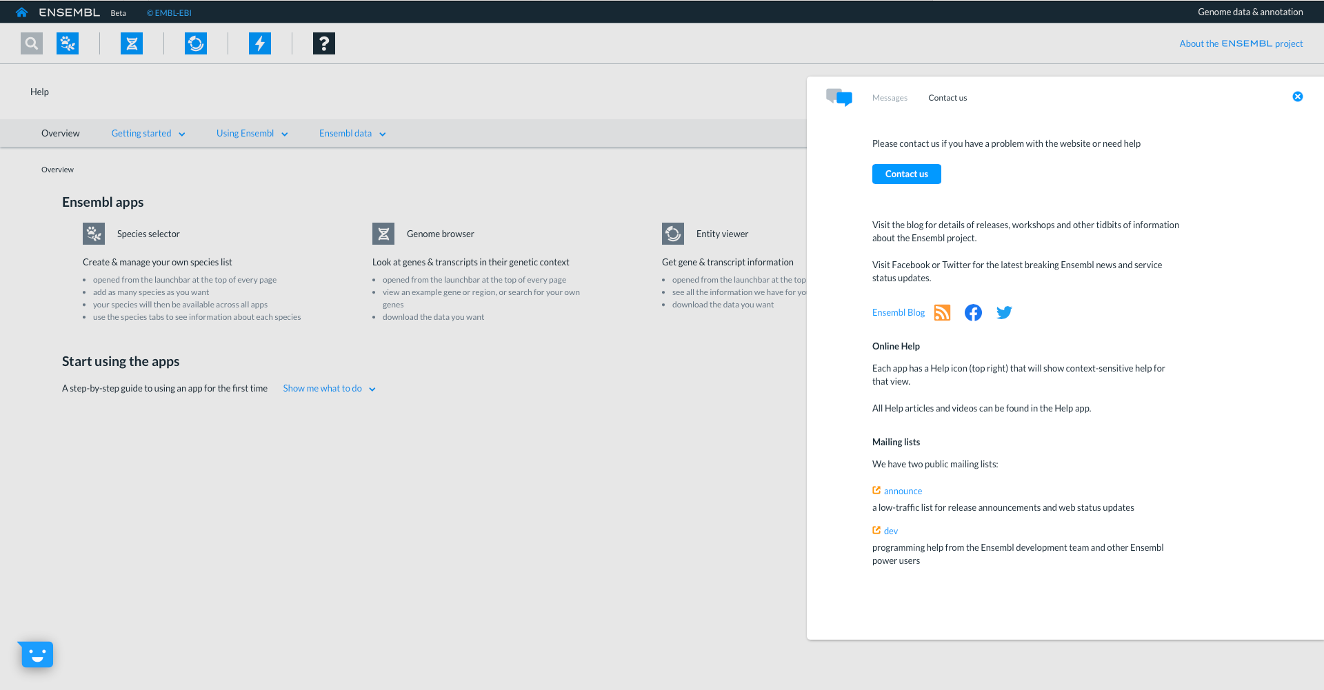
You will also find a ‘contact us’ icon on the top right of every page where you can get In touch to leave more detailed feedback or ask questions. Links to the blog, our social media and mailing lists are also provided.
Variation
In any of the sequence views shown in the Gene and Transcript tabs, you can view variants on the sequence. You can do this by clicking on Configure this page from any of these views.
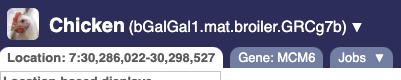
Let’s take a look at the Gene sequence view for MCM6 in chicken. Search for MCM6 and go to the Sequence view.
If you can’t see variants marked on this view, click on Configure this page and select Show variants: Yes and show links.
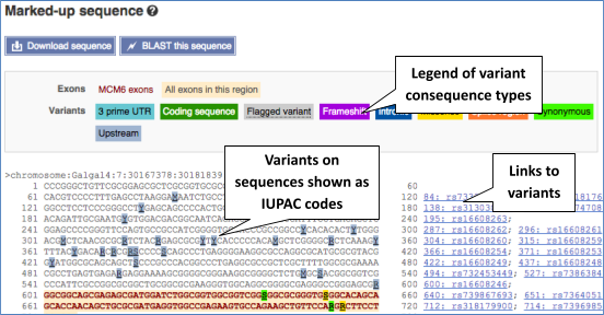
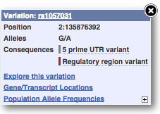
Find out more about a variant by clicking on it.
You can add variants to all other sequence views in the same way.
You can go to the Variation tab by clicking on the variant ID. For now, we’ll explore more ways of finding variants.
To view all the sequence variations in table form, click the Variant table link at the left of the gene tab.
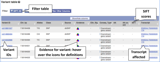
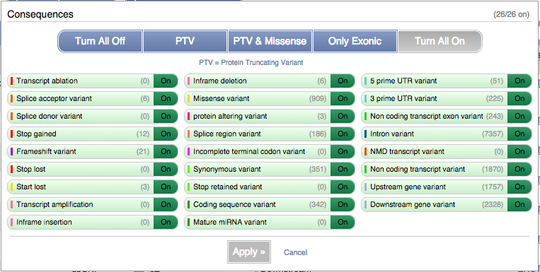
You can filter the table to only show the variants you’re interested in. For example, click on Consequences: All, then select the variant consequences you’re interested in.
You can also filter by SIFT, or click on Filter other columns for filtering by other columns such as Evidence or Class.
The table contains lots of information about the variants. You can click on the IDs here to go to the Variation tab too.
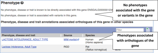
You can also see the phenotypes associated with a gene. Click on Phenotype in the left hand menu.
Let’s have a look at variants in the Location tab. Click on the Location tab in the top bar.
Click on Configure this page and open Variation from the left-hand menu.
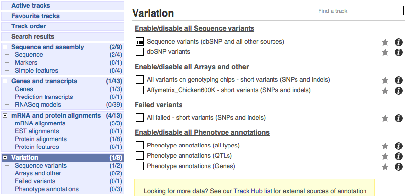
There are various options for turning on variants. You can turn on variants by source, by frequency, presence of a phenotype or by individual genome they were isolated from. You can also turn on QTLs, which cover a locus without being associated with a specific variant. Turn on the following variation tracks.
- All variants on genotyping chips - short variants (SNPs and indels)
- Phenotype annotations (QTLs)

Click on a variant to find out more information. It may be easier to see the individual variants if you zoom in.
Let’s have a look at a specific variant, which happens to fall within the MCM6 gene: rs14625781.
The easiest way to find this variant is if we put rs14625781 into the search box. Click through to open the Variation tab.
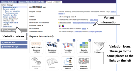
The icons show you what information is available for this variant. Click on Genes and regulation, or follow the link at the left.
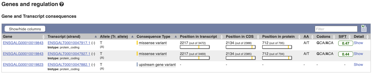
This variant is found in three transcripts of the MCM6 gene, and is missense in two. SIFT predicts that it is unlikely to affect protein function of either (Tolerated).
Let’s look at population genetics. Either click on Explore this variant in the left hand menu then click on the Population genetics icon, or click on Population genetics in the left-hand menu.
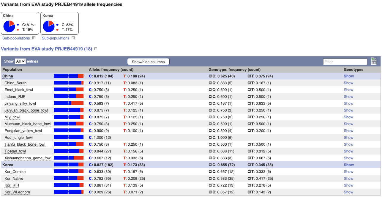
We can see data from EVA study PRJEB44919 showing the frequency of the alleles and genotypes. We can see what animals these genotypes were actually observed in by going to Sample genotypes.
Click on Phylogenetic context to see the variant in other species.
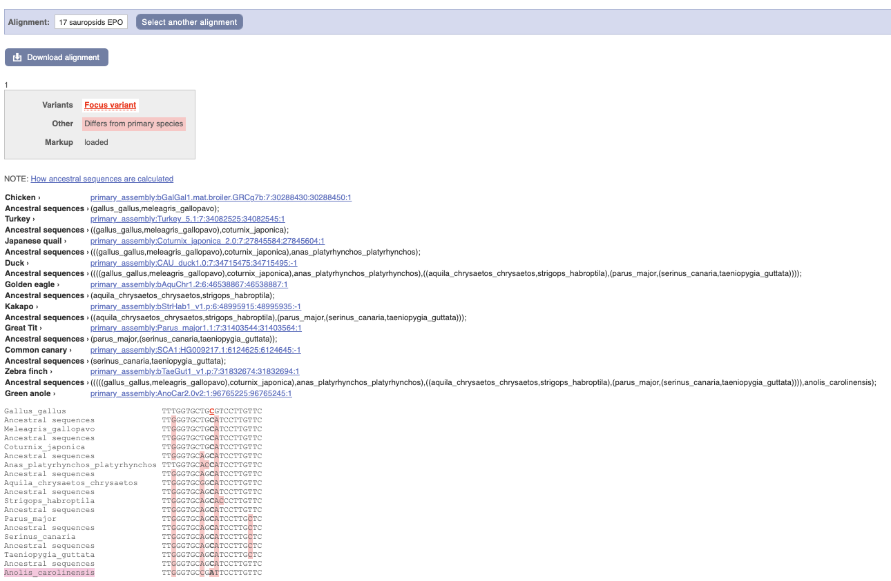
We can see that other birds also have the C alleles as a reference whereas Anolis_carolinensis has an A allele.
Exploring a SNP in chicken
(a) Find the page with information for the chicken SNP rs10731268.
(b) What gene(s) does rs10731268 fall within? What is its effect?
(c) Have any papers been written mentioning rs10731268? What are they about?
(d) What allele is at this position in other birds? What is the likely ancestral allele?
(a) Go to the Ensembl homepage.
Type rs10731268 in the Search box, then click Go. Click on rs10731268.
(b) Click on Genes and Regulation in the side menu (or the Genes and Regulation icon).
rs10731268 falls within 2 genes: ENSGALG00010028562 and ENSGALG00010028568 (HGNC: MLLT1). This variant has a missense consequence in seven transcripts of the ENSGALG00010028562 gene, and downstream gene variant consequence in three transcripts of the ENSGALG00010028568 (HGNC: MLLT1) gene.
(c) Click on Citations in the left hand side menu.
This variant is mentioned in the paper ‘Identification and characterization of genes that control fat deposition in chickens’ from 2013 by D’Andre et al. Click on the PubMed ID 24206759 to go to the paper.
(d) Click on Phylogenetic Context in the side menu. Select Alignment: 17 sauropsids EPO and click Go.
Japanese quail, Duck, Golden Eagle, Common canary and Zebra finch all have an A in this position. This suggests that A may be the ancestral allele.
Exploring a variant in pig
The human gene MC4R has been associated with obesity. The SNP rs81219178 has been identified as a variant in the pig MC4R gene.
(a) What is the amino acid change caused by rs81219178 in MC4R of the pig? Is the change likely to alter the protein function?
(b) How many transcripts does this variant affect? What are the consequences of this variant?
(a) Go to the Ensembl homepage.
Type rs81219178 in the Search box, then click Go.
Click on rs81219178 (Pig Variant, Breed: reference).
Click on Genes and regulation in the left-hand menu or on the icon.
The variant causes a D->N amino acid change (Aspartic acid -> Asparagine). The SIFT score of 0.01 predicts that this change will have a deleterious effect on the protein.
(b) This variant affects one transcript (ENSSSCT00000091644.1) of ENSSSCG00000051798 gene and it has the missense consequence.
Ensembl VEP
We have identified seven variants in pig:
rs319195925, rs80805426, rs81267388, rs80854621, rs711163915, rs321793337, rs792403417
We will use the Ensembl VEP to determine:
- If the variants have been annotated in Ensembl already
- If genes are affected by the variants
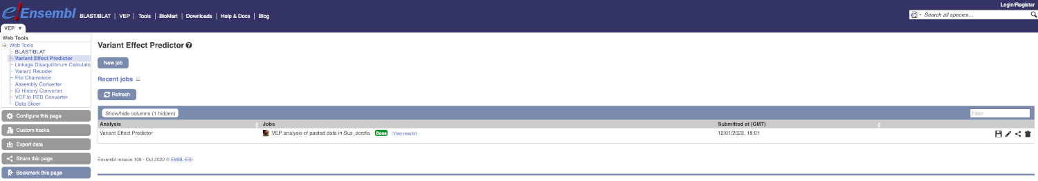
Go to the front page of Ensembl and click on Variant Effect Predictor in the Tools section or click on VEP in the top header.
This page contains information about the VEP, including a link for downloading the script version of the tool. Click on the Launch VEP button to open the input form.
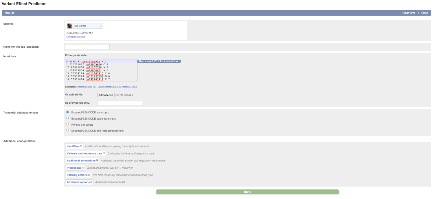
Lets input the variants data in VCF format:
Chromosome Position Name Reference Alternative
Put the following into the Input data box:
9 9580742 rs319195925 T C
1 213701082 rs80805426 C A
15 83361856 rs81267388 A G
1 159538854 rs80854621 A G
14 50574184 rs711163915 C A
14 50571223 rs321793337 G A
14 50571474 rs792403417 C T
The VEP will detect automatically that the data is in VCF format.
There are further options that you can choose for your output. These are categorised as Identifiers, Variants and frequency data, Additional annotation, Predictions, Filtering options and Advanced options. Let’s open all menus and take a look.
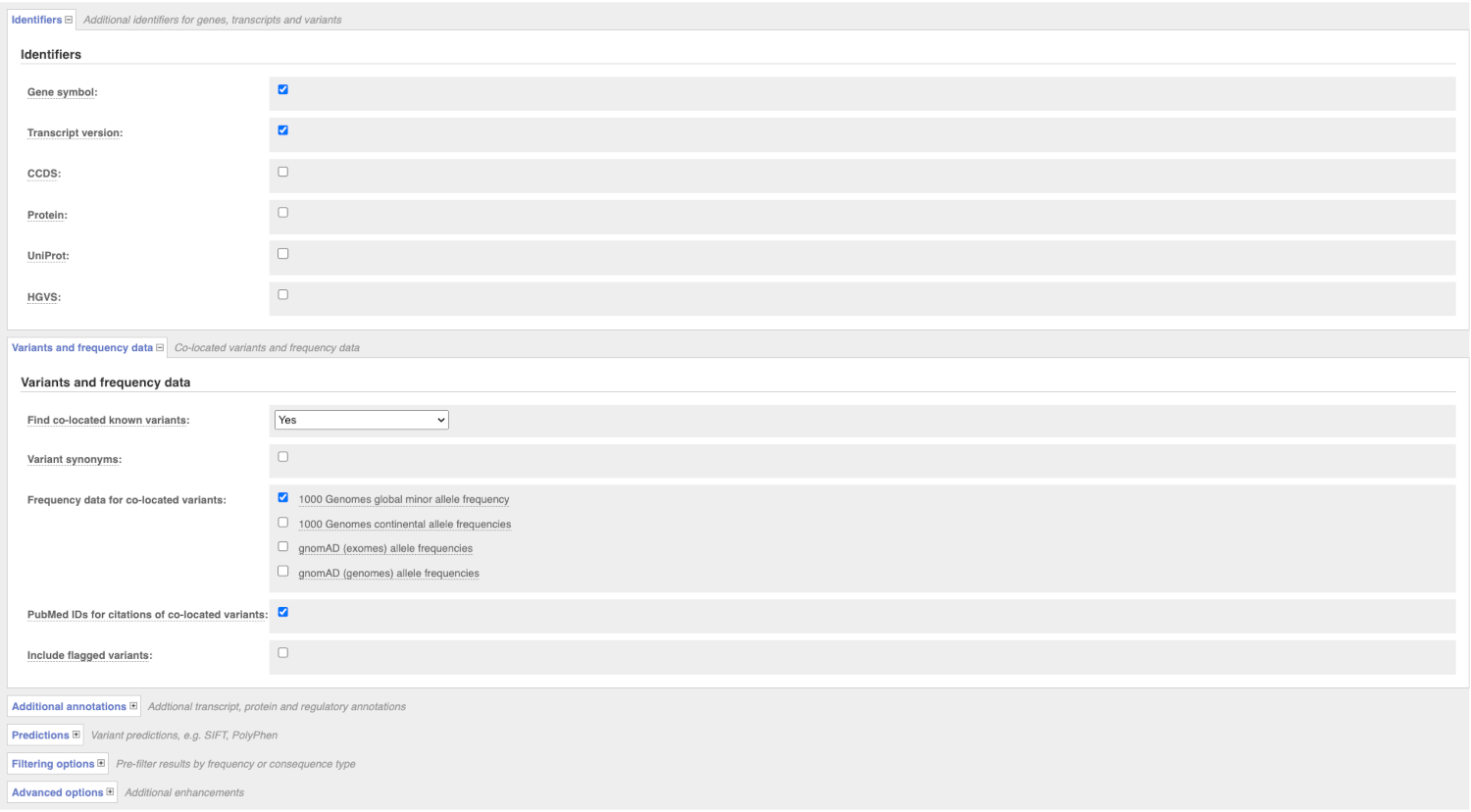
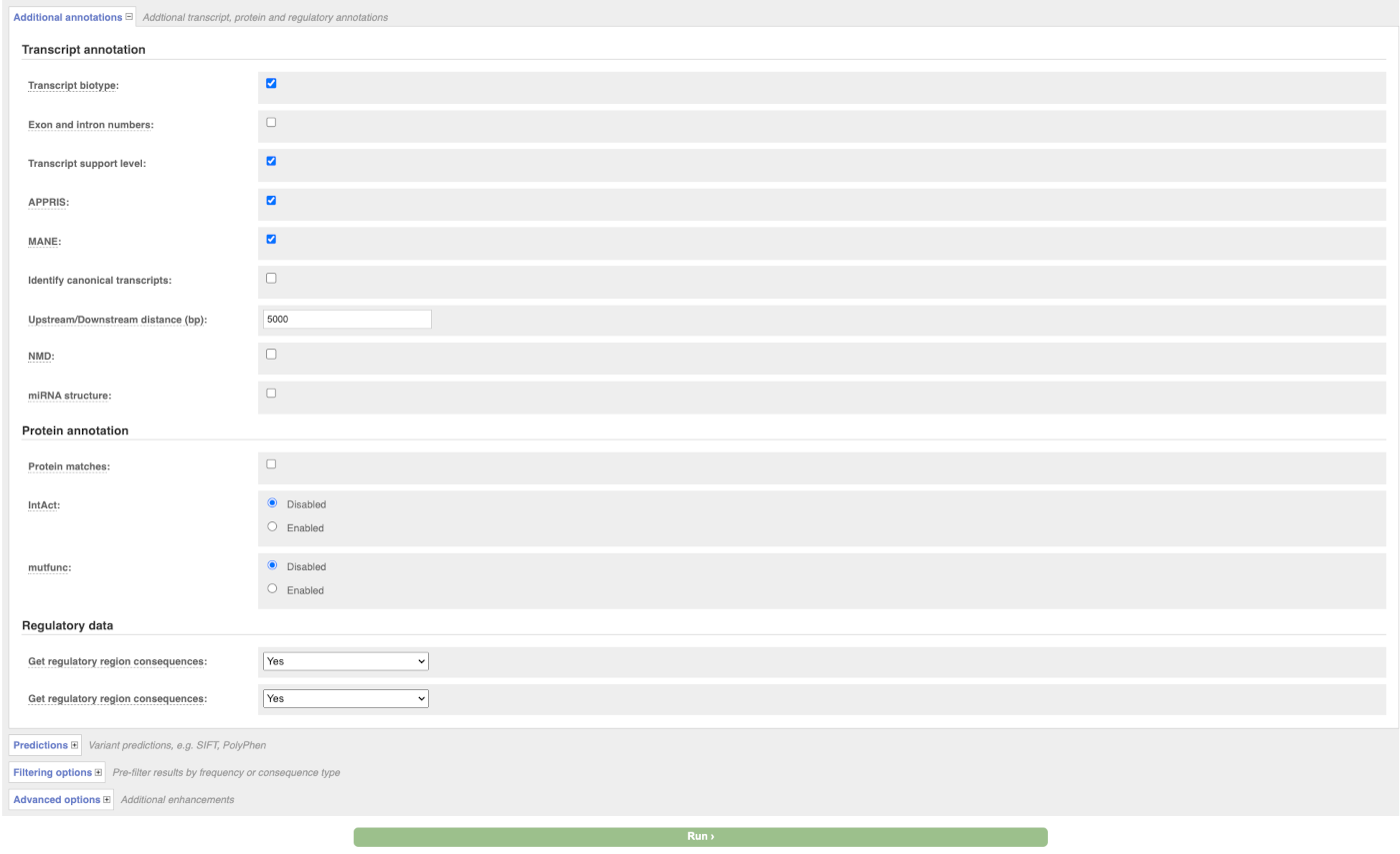
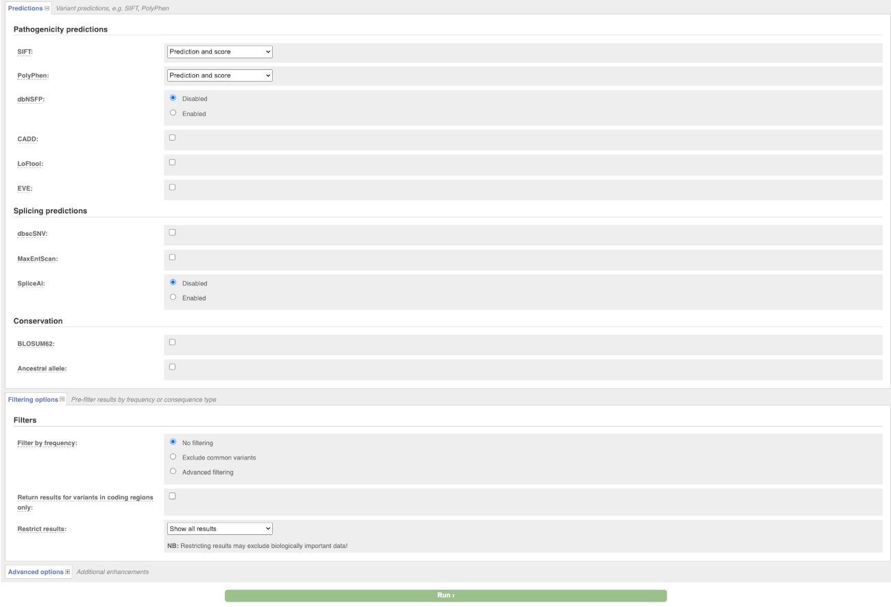
Hover over the options to see definitions.
When you have selected everything you need, scroll right to the bottom and click Run.
The display will show you the status of your job. It will say Queued, then automatically switch to Done when the job is done, you do not need to refresh the page. You can save, edit, share or delete your job at this time. If you have submitted multiple jobs, they will all appear here.
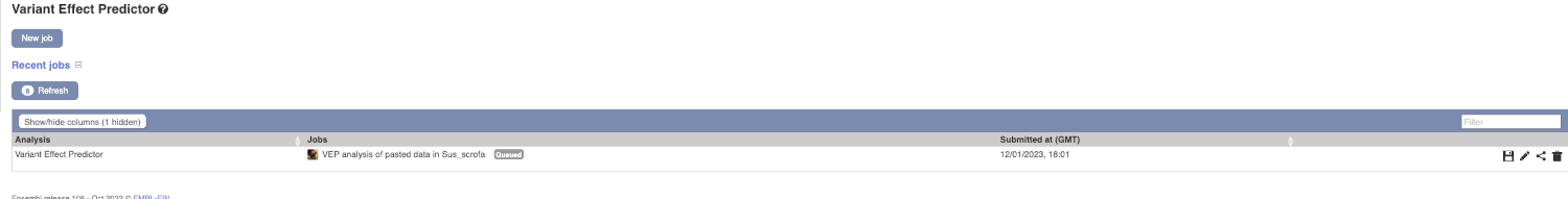
Click on View Results once your job is done.
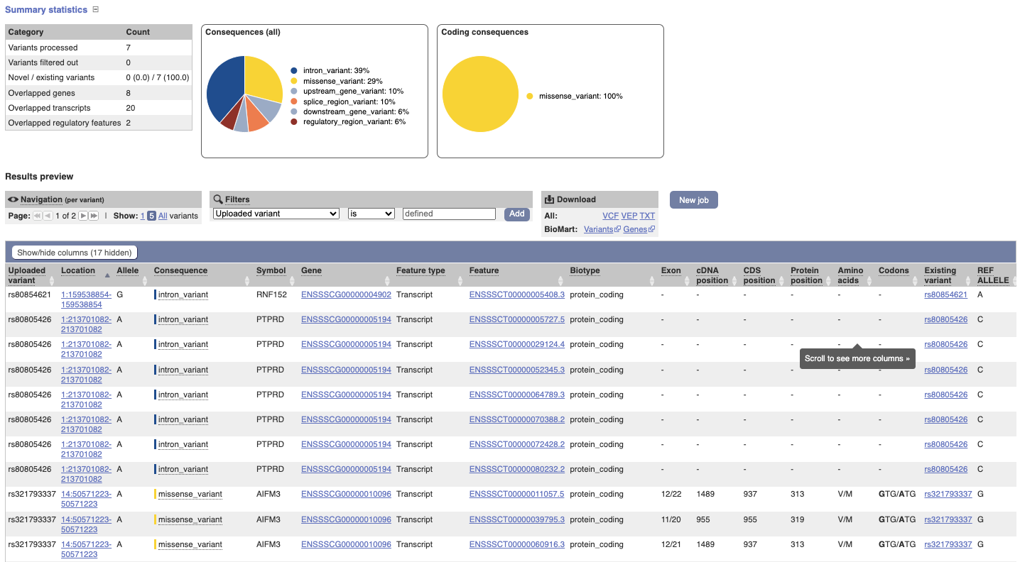
In your results you will see a graphical and table summary of the data as well as a table with the detailed results.
VEP for chicken data
We have identified a few variants associated with body size in chicken (bGalGal1.mat.broiler.GRCg7b):
chr 6, genomic coordinate 23650222, alleles A/C, forward strand
chr 6, genomic coordinate 23645685, alleles C/A, forward strand
chr 1, genomic coordinate 51237121, alleles C/T, forward strand
(a) Which genes and transcripts do these variants map to?
(b) What are the consequence terms for these variants?
(c) Which regulatory feature is affected by the variants?
Go to the Variant Effect Predictor (VEP) under Tools on the top banner of any Ensembl page.
Copy the following into the Paste data text box: 6 23650222 23650222 A/C + var1, 6 23645685 23645685 C/A + var2, 1 51237121 51237121 C/T + var3,
Note that this is the Ensembl default format (chr start end reference/alternate alleles). For additional formats accepted by VEP, have a look here: http://www.ensembl.org/info/docs/tools/vep/vep_formats.html
Click Run.
(a) In the Results table, you’ll see that the variants fall into three genes.
(b) The consequence terms are listed in the Consequence column and Consequences (all) chart and include intron_variant, regulatory_region_variant, upstream_gene_variant and downstream_gene_variant.
(c) Variant 3 at 1:51237121-51237121 with T allele affects regulatory feature ENSR00000006264 (promoter).
BioMart
Follow these instructions to guide you through BioMart to answer the following query:
You have three questions about a set of chicken genes:
ESPN, MYH9, USH1C, CISD2, THRB, WHRN
(these are HGNC gene symbols. More details on the HUGO Gene Nomenclature Committee can be found on https://www.genenames.org/)
- What are the NCBI Gene IDs for these genes?
- Are there associated functions from the GO (gene ontology) project that might help describe their function?
- What are their cDNA sequences?
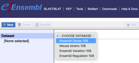
Click on BioMart in the top header of the Ensembl website or go to BioMart directly by visiting https://www.ensembl.org/biomart/martview.
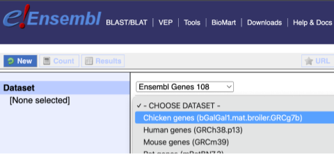
You cannot choose any filters or attributes until you’ve chosen your dataset. Your dataset is the data type you’re working with. In this case we’re going to choose genes, so pick Ensembl Genes then Chicken genes from the drop-downs.
Now that you’ve chosen your dataset, the filters and attributes will appear in the column on the left. You can pick these in any order and the options you pick will appear.
Click on Filters on the left to see the available filters appear on the main page. You’ll see that there are loads of categories of Filters to choose from. You can expand these by clicking on them. For our query, we’re going to expand GENE.
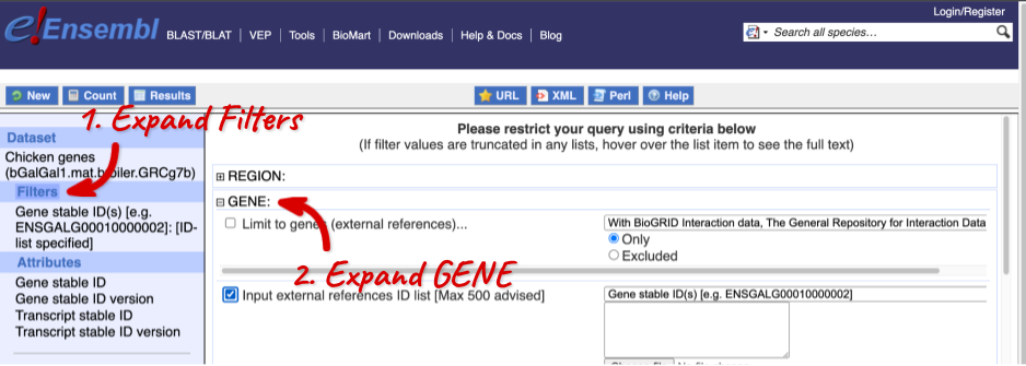
Our input data is a list of identifiers, so we’re going to use the Input external references ID list filter. This allows us to input a list of identifiers from different databases. We need to choose what kind of identifier we’re using, so that BioMart can look up the right column in a data table. You can pick these from a drop-down list, which lists the type of identifier with an example of how it looks. For our query, we have a list of gene names, so we need to pick Gene Name(s).

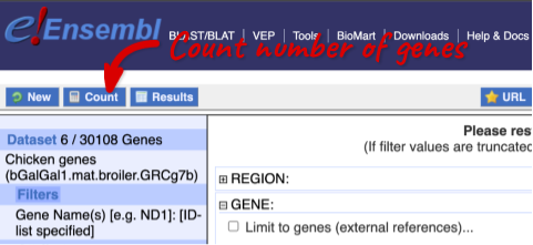
To check if the filters have worked, you can use the Count button at the top left, which will show you how many genes have passed the filter. If you get 0 or another number you don’t expect, this can help you to see if your query was effective.
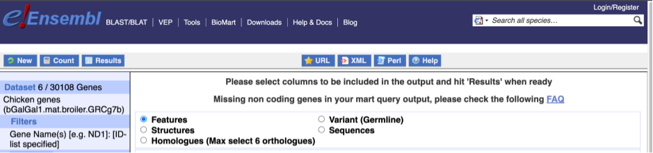
To choose the attributes, expand this in the menu. There are six categories for chicken gene attributes. These categories are mutually exclusive, you cannot pick attributes from multiple categories. This means that we need to do two separate queries to get our GO terms and NCBI IDs, and to get our cDNA sequences.
The Ensembl gene and transcript IDs, with and without version numbers are selected by default. The selected attributes are also listed on the left.
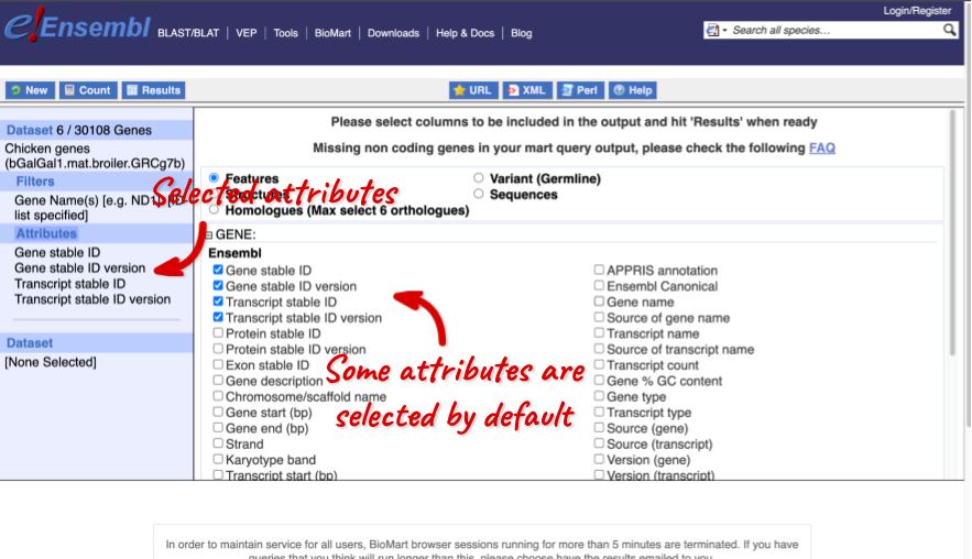
We can choose the attributes we want by clicking on them. For our query, we’re going to select:
- GENE
- Gene Name
- EXTERNAL
- NCBI gene ID
- GO term accession
- GO term name
- GO term definition
We need to select the Gene Name in order to get back our original input, as this is not returned by default in BioMart. The order that you select the attributes in will define the order that the columns appear in in your output table.
You can get your results by clicking on Results at the top left.
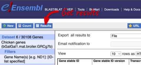
The results table just gives you a preview of the first ten lines of your query. This allows the results to load quickly, so that if you need to make any changes to your query, you don’t waste any time. To see the full table you can click on View ## rows. You can also export the data to an xls, tsv, csv or html file. For large queries, it is recommended that you export your data as Compressed web file (notify by email), to ensure your download is not disrupted by connection issues.
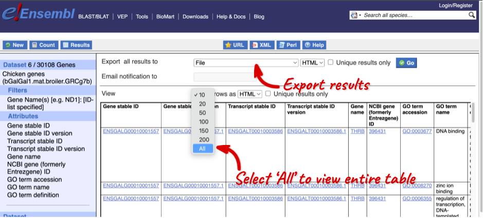
You can see multiple rows per gene in your input list, because there are multiple transcripts per gene and multiple GO terms per transcript.
To get the cDNA sequences, go back to the Attributes then select the category Sequences and expand SEQUENCES.
When you select the sequence type, the part of the transcript model you’ve chosen will be highlighted in the grpahic.
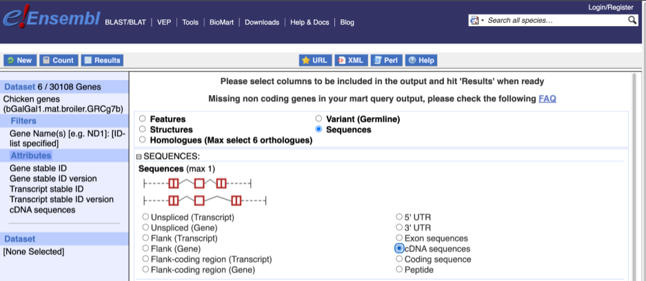
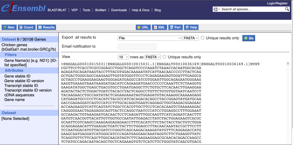
Choose cDNA sequences, then expand HEADER INFORMATION to add Gene Name to the header. Then hit Results again.
For more details on BioMart, have a look at this publication: Kinsella RJ, Kähäri A, Haider S, et al. Ensembl BioMarts: a hub for data retrieval across taxonomic space. Database: the Journal of Biological Databases and Curation. 2011; 2011:bar030. DOI: 10.1093/database/bar030. PMID: 21785142; PMCID: PMC3170168.
BioMart: Convert IDs
BioMart is a very handy tool when you want to convert IDs from different databases. The following is a list of 27 IDs of Sus scrofa proteins from the NCBI RefSeq database: NP_001116455,NP_001231885,NP_001230616,NP_001231413,NP_001231746,NP_999129,NP_001231602,NP_001177096,NP_001231419,NP_001230512, NP_001231165,NP_001167636,NP_001172069,NP_001011509,NP_999191,NP_001231786,NP_001231468,NP_001121951,NP_001230557,NP_999413
Generate a list that shows to which Ensembl Gene IDs and to which gene names these RefSeq IDs correspond. Do these 27 proteins correspond to 27 genes?
Click New. Choose the ENSEMBL Genes database. Choose the Pig genes (Sscrofa11.1) dataset.
Click on Filters in the left panel. Expand the GENE section by clicking on the + box. Select Input external references ID list - RefSeq peptide ID(s) and enter the list of IDs in the text box (either comma separated or as a list). HINT: You may have to scroll down the menu to see these. Count shows 20 genes.
Click on Attributes in the left panel. Select the Features attributes page. Expand the GENE tab by clicking on the + box. Select Gene name. Expand the EXTERNAL tab. Select RefSeq Peptide ID.
Click the Results button on the toolbar. Select View All rows as HTML or export all results to a file.
BioMart: Finding genes by protein domain
Find chicken proteins with transmembrane domains located on chromosome 9.
As with all BioMart queries you must select the dataset, set your filters (input) and define your attributes (desired output). For this exercise:
Dataset: Ensembl genes in chicken
Filters: Transmembrane proteins on chromosome 9
Attributes: Ensembl gene and transcript IDs and Associated gene names
Go to the Ensembl homepage (https://www.ensembl.org) and click on BioMart at the top of the page. Select Ensembl genes as your database and Chicken genes (bGalGal1.mat.broiler.GRCg7b) as the dataset. Click on Filters on the left of the screen and expand REGION. Change the chromosome to 9. Now expand PROTEIN DOMAINS AND FAMILIES, also under filters, and select Limit to genes …, choosing With Transmembrane helices from the drop-down and select Only. Clicking on Count should reveal that you have filtered the dataset down to 143 genes.
Click on Attributes. Under Features expand GENE. Select Gene name.
Now click on Results. The first 10 results are displayed by default; display all results by selecting All from the drop-down menu above the table.
The output will display the Ensembl gene ID, Ensembl Transcript ID and associated gene names of all proteins with a transmembrane domain on chicken chromosome 9. If you prefer, you can also export as an Excel sheet by using the Export all results to XLS option.
BioMart: Find genes associated with array probes
Here are two affymetrix probeset IDs from my microarray experiment that seem to map uniquely to genes in the chicken genome: Gga.12669.1.S1_at, GgaAffx.7784.1.S1_at
(a) Retrieve for the genes corresponding to these probe-sets the Ensembl Gene and Transcript IDs as well as their gene symbols and descriptions.
(b) In order to analyse these genes for possible promoter/enhancer elements, retrieve the 2000 bp upstream of the transcripts of these genes.
(c) In order to be able to study these chicken genes in duck, identify their duck orthologues. Also retrieve the genomic coordinates of these orthologues.
(a) Click New. Choose the Ensembl Genes database. Choose the Chicken genes dataset.
Click on Filters in the left panel. Expand the GENE section by clicking on the + box. Select Input microarray probes/probesets ID list - AFFY Chicken probe ID(s) and enter the list of probeset IDs in the text box (either comma separated or as a list).
Count shows three genes match this list of probesets.
Click on Attributes in the left panel. Select the Features attributes page. Expand the GENE section by clicking on the + box. In addition to the default selected attributes, select Gene name and Gene description. Expand the EXTERNAL section by clicking on the + box. Select AFFY Chicken probe from the Microarray probes/probesets section.
Click the Results button on the toolbar. Select View All rows as HTML or export all results to a file. Tick the box Unique results only.
Your results should show that the 2 probes map to 2 Ensembl genes.
(b) Don’t change Dataset and Filters – simply click on Attributes.
Select the Sequences category. Expand the SEQUENCES tab by clicking on the + box. Select Flank (Transcript) and enter 2000 in the Upstream flank text box. Expand the HEADER INFORMATION tab by clicking on the + box. Select Gene description and Gene name in addition to the default selected attributes.
Note: Flank (Transcript) will give the flanks for all transcripts of a gene with multiple transcripts. Flank (Gene) will give the flanks for one possible transcript in a gene (the most 5’ coordinates for upstream flanking).
Click the Results button on the toolbar.
(c) You can leave the Dataset and Filters the same, and go directly to the Attributes section:
Click on Attributes in the left panel. Select the Homologues category. Expand the GENE tab by clicking on the + box. Select Gene name. Unselect Transcript stable ID and Transcript stable ID version. Expand the ORTHOLOGUES [A-E] tab by clicking on the + box. Select Duck gene stable ID, Duck chromosomes/scaffold name, Duck chromosome/scaffold start (bp) and Duck chromosome/scaffold end (bp).
Click the Results button on the toolbar. Select View All rows as HTML or export all results to a file.
Your results should show that for each chicken gene, one duck orthologue has been identified.