Filter Events by Year
Ensembl Plants Browser Workshop - International Master in Plant Genetics, Genomics and Breeding, IAMZ-CIHEAM
Course Details
- Lead Trainer
- Louisse Paola Mirabueno
- Associate Trainer(s)
-
- Bruno Contreras Moreira
- Ricardo Ramírez
- Event Dates
- 2023-12-14 until 2023-12-15
- Location
- CIHEAM, Zaragoza, Spain
- Description
- Work with the Ensembl Outreach team to get to grips with the Ensembl Plants browser.
Demos and exercises
Variation
Exploring variants in rice
Visualising variants in the Sequence view
In any of the sequence views shown in the Gene and Transcript tabs, you can view variants on the sequence. You can do this by clicking on Configure this page from any of these views.
Let’s take a look at the Gene sequence view for OS01G0775500 in rice. Search for OS01G0775500 and go to the Sequence view.
If you can’t see variants marked on this view, click on Configure this page and select Show variants: Yes and show links.
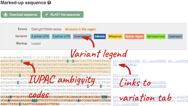
Find out more about a variant by clicking on it.
You can add variants to all other sequence views in the same way.
You can go to the Variation tab by clicking on the variant ID. For now, we’ll explore more ways of finding variants.
Viewing variants within a gene in the tabular form
To view all the sequence variants in table form, click the Variant table link at the left of the gene tab.
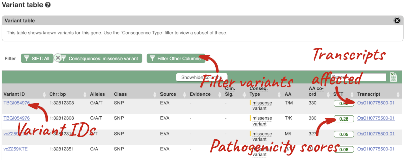
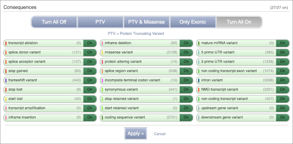
You can filter the table to only show the variants you’re interested in. For example, click on Consequences: All, then select the variant consequences you’re interested in. For display purposes, the table above has already been filtered to only show missense variants.
You can also filter by the different pathogenicity scores and MAF, or click on Filter other columns for filtering by other columns such as Evidence or Class.
The table contains lots of information about the variants. You can click on the IDs here to go to the Variation tab too.
Visualising variants in the Region in Detail view
Let’s have a look at variants in the Location tab. Click on the Location tab in the top bar.
Configure this page and open Variation from the left-hand menu.
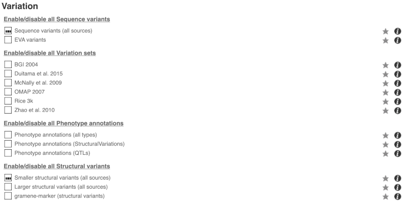
There are various options for turning on variants. You can turn on variants by source, by frequency, presence of a phenotype or by individual genome they were isolated from. You can also turn on genotyping chips.
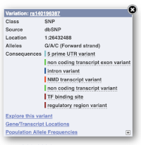
Exploring a specific variant
Let’s have a look at a specific variant. If we zoomed in we could see the variant rs18335701 in this region, however it’s easier to find if we put rs18335701 into the search box. Click through to open the Variation tab for Oryza sativa Japonica.
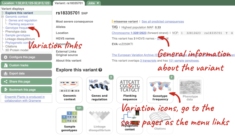
The icons show you what information is available for this variant. Click on Genes and regulation, or follow the link on the left.
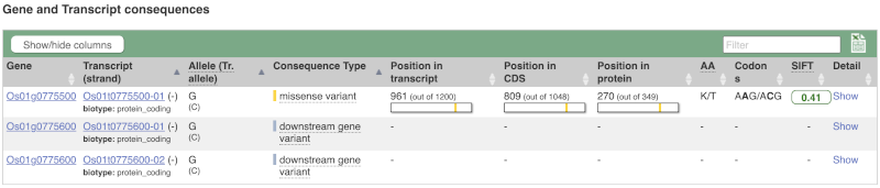
This page illustrates the genes the variant falls within and the consequences on those genes, including pathogenicity predictors. It also shows data from GTEx on genes that have increased/decreased expression in individuals with this variant, in different tissues. Finally, regulatory features and motifs that the variant falls within are shown.
Let’s look at population genetics. Click on Population genetics in the left-hand menu.
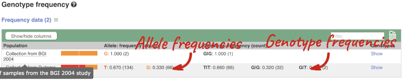
The population allele frequencies are shown by study. Where genotype frequencies are available, these are shown in the tables.
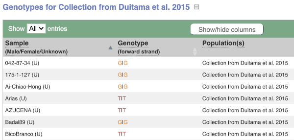
We can see which strains these genotypes were observed in by going to Sample Genotypes. Click on Show for the Duitama et al. 2015 population.
Exploring a SNP in Arabidopsis
The Arabidopsis thaliana ATCDSP32 protein is a chloroplastic drought-induced stress protein proposed to participate in a process called cell redox homeostasis. Go to Ensembl Plants and answer the following questions:
-
How many variants have been identified in the gene that can cause a change in the protein sequence (i.e. missense variant)?
-
What is the ID of the variant that changes the amino acid residue 60 from Alanine to Threonine (hint: refer to an amino acid codon table)? What is the location of this SNP in the A. thaliana genome? What are its possible alleles?
-
Download the flanking sequence of this SNP in RTF (Rich Text Format). Can you change how much flanking sequence is displayed on the browser?
-
Does this SNP cause a change at the amino acid level for other genes or transcripts?
- Click on Arabidospsis thaliana on the Ensembl Plants homepage. Search for ATCDSP32 on the species page and in the search results, click on the Gene ID AT1G76080. In the left-hand side menu of the Gene tab, click on Variant table. Click on Consequences: All then select only missense variant.
The missense variant button indicates that there are 18 of these. Alternatively, you can count the number of variants in your filtered list.
- An amino acid codon table can be found on Wikipedia. Sort the AA coord column by clicking on the header and scroll down to find a variant at residue 60. The ID of this variant is ENSVATH05153232.
The variant is located at position 28549171 on chromosome 1. The two possible alleles at this locus are C (reference) and T (alternative).
- Click on the link ENSVATH05153232, then click on Flanking sequence in the left-hand side menu. Now click on Download sequence and select File format > Rich Text Format (RTF).
If you want to change how much flanking sequence is displayed on the browser, go back to the Flanking sequence page, click on the Configuration button and change the length of the sequence. The default settings is 400 bp.
- Click on Genes and regulation in the left-hand side menu.
This SNP does not cause a change at the amino acid level for any other genes or transcripts in A. thaliana.
Variation data in tomato
-
Go to Ensembl Plants and find the Solyc02g084570.3 gene in Solanum lycopersicum (tomato) and go to its Location tab. Can you see the variation track?
-
Zoom in around the last exon of this gene. What are the different types of variants seen in that region? Are any splice region variants mapped in the region? If so, what is/are the coordinate(s)?
- Select Solanum lycopersicum from the Species search drop-down menu and search for
Solyc02g084570.3. In the results page, you can click on the coordinates 2:48284598-48288482 to go straight to the Location tab. Scroll down to the Region in detail view. The variation track is shown at the bottom of the view.If you don’t see the Variation - All sources track, click Configure this page on the left-hand panel, search for the track in the pop-up menu and enable the track by clicking on the square next to the track name. Close the pop-up window and wait for the track to load.
- Zoom in around the last exon of this gene by drawing a box in the respective region (you can change your mouse action by clicking the Drag/Select icons at the top right-hand corner of the view). Note the gene is on the reverse strand (this is signified by the < sign next to the transcript name, and it is located below the Contigs track), so the last exon will be on the left hand side of that image. The variation legend is shown at the bottom of the page, telling you what the colours mean.
The types of variants seen in that region are 3’ UTR, missense, synonymous and splice region variants.
Splice region variants are shown in orange. Click on the variants to get additional information on that variant including location. You can zoom into the region if the variant block is too small to click.
The variants are found at 2:48285642 and 2:48285640-48285641. Note that the two variants overlap: one is a SNP and the other is an indel. SNPs are tagged with ambiguity codes (zoom into the region if you cannot see this). You can find a useful IUPAC ambiguity code guid on the bioinformatics.org website. Single-letter ambiguity codes are given when two or more possible nucleotides may be represented at a single base locus.
Investigating a variant in wheat
-
Search for the variant
BA00369602in Triticum aestivum on Ensembl Plants. Is this variant known by any other names? -
What gene is affected by this variant? What is the amino acid change?
-
Which cultivars have the alternative base at this locus?
- Start at the homepage and enter BA00369602 into the search box and select Triticum aestivum from the drop-down list. Click on the Gene ID BA00369602 in the search results to get to the variation homepage.
Under Synonyms, you can see that the variant is also known as AX-94448191 in CerealsDB.
- Click on Genes and regulation.
The variant is a missense variant on TraesCS2D02G303800, where it gives a glycine to aspartic acid (G/D) change at transcript position 406.
- Click on Sample genotypes. Scroll down the table to see if there are any cultivars with the A allele in the genotype column.
All of the cultivars listed have the genotype
G|G.
VEP
Demonstration of the VEP web interface
Input
We have identified three variants on wheat chromosome 4B:
C -> T at 240206468
C -> G at 240199078
C -> T at 240212229
We will use the Ensembl VEP to determine:
- Have my variants already been annotated in Ensembl?
- What genes are affected by my variants?
- Do any of my variants affect gene regulation?
Click on Tools in the top green bar from any Ensembl Plants page, then Variant Effect Predictor to open the input form:
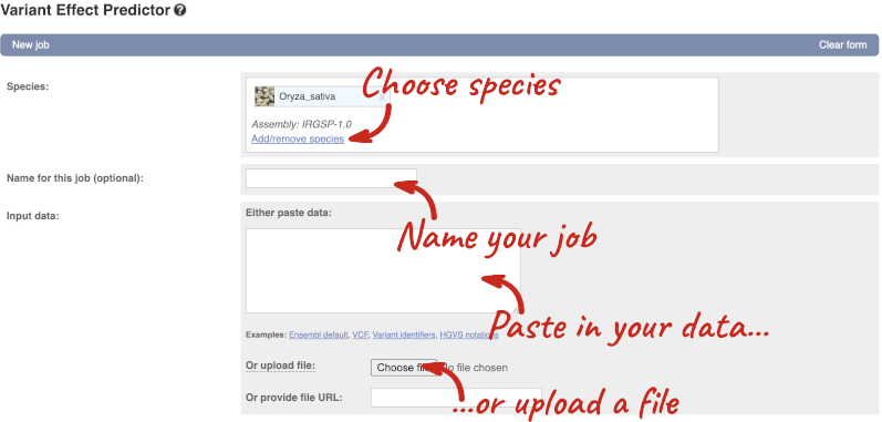
Click on Add/remove species and search for Triticum aestivum to choose it.
The data is in VCF:
chromosome coordinate id reference alternative
Put the following into the Paste data box:
4B 240206468 var1 C T
4B 240199078 var2 C G
4B 240212229 var3 C T
The VEP will automatically detect that the data is in VCF.
Additional configurations
There are further options that you can choose for your output. These are categorised as Identifiers, Variants and frequency data, Additional annotations, Predictions, Filtering options and Advanced options. Let’s open all the menus and take a look.
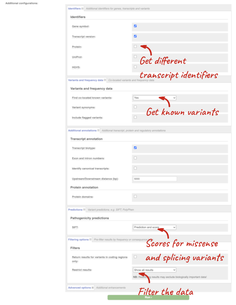
Hover over the options to see definitions.
When you’ve selected everything you need, scroll right to the bottom and click Run.

The display will show you the status of your job. It will say Queued, then automatically switch to Done when the job is done, you do not need to refresh the page. You can edit or discard your job at this time. If you have submitted multiple jobs, they will all appear here.
Click View results once your job is done.
Results
In your results you will see a graphical summary of your data, as well as a table of your results.
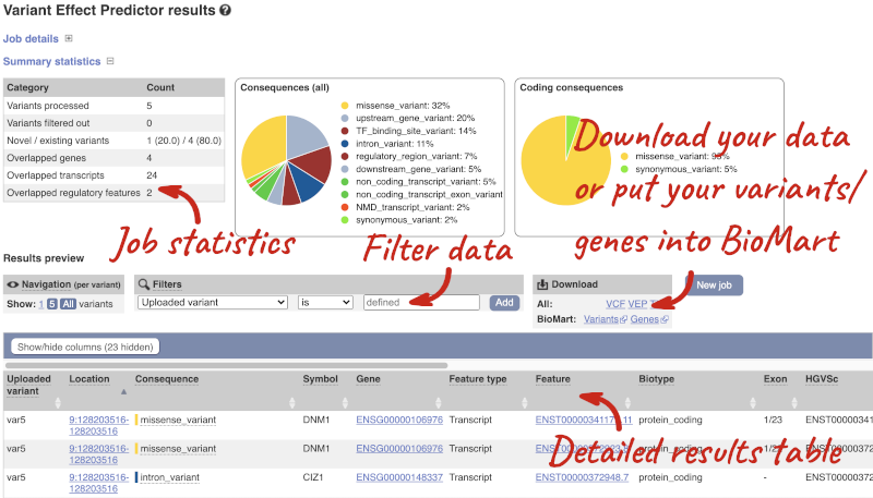
The results table is enormous and detailed, so we’re going to go through the it by section. The first column is Uploaded variant. If your input data contains IDs, like ours does, the ID is listed here. If your input data is only loci, this column will contain the locus and alleles of the variant. You’ll notice that the variants are not neccessarily in the order they were in in your input. You’ll also see that there are multiple lines in the table for each variant, with each line representing one transcript or other feature the variant affects.
You can mouse over any column name to get a definition of what is shown.
The next few columns give the information about the feature the variant affects, including the consequence. Where the feature is a transcript, you will see the gene symbol and stable ID and the transcript stable ID and biotype. The IDs are links to take you to the gene or transcript homepage.
This is followed by details on the effects on transcripts, including the position of the variant in terms of the exon number, cDNA, CDS and protein, the amino acid and codon change and pathogenicity scores. Where the variant is known, the ID of the existing variant is listed, with a link out to the variant homepage. The pathogenicity scores are shown as numbers with coloured highlights to indicate the prediction, and you can mouse-over the scores to get the prediction in words.
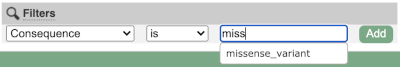
Above the table is the Filter option, which allows you to filter by any column in the table. You can select a column from the drop-down, then a logic option from the next drop-down, then type in your filter to the following box. We’ll try a filter of Consequence, followed by is then missense_variant, which will give us only variants that change the amino acid sequence of the protein. You’ll notice that as you type missense_variant, the VEP will make suggestions for an autocomplete.
You can export your VEP results in various formats, including VCF. When you export as VCF, you’ll get all the VEP annotation listed under CSQ in the INFO column. After filtering your data, you’ll see that you have the option to export only the filtered data. You can also drop all the genes you’ve found into the Gene BioMart, or all the known variants into the Variation BioMart to export further information about them.
Running command-line VEP via Docker
If you don’t have root privileges, you can run VEP in a virtualised container via Docker. You can download and install Docker on Mac, Windows and Linux.
Preparing and running Docker
You will need to install or update Rosetta 2 to run Docker:
softwareupdate --install-rosetta
Create a directory for the course:
mkdir /Desktop/VEP/Plants
cd /Desktop/VEP/Plants
Start Docker:
open –a Docker
Download the Ensembl Plants VEP Docker image:
docker pull csicunam/bioinformatics_iamz
Create a Docker working directory to mount to the Docker image (you can save your input files in here and all outputs will be written in this directory):
mkdir vep_data
Some operating systems may require root privileges:
chmod 777 vep_data
Run the Docker image and mount the directory you just created:
docker run -t -i -v $HOME/Desktop/VEP/Plants/vep_data:/data csicunam/bioinformatics_iamz:latest
Exit Docker
exit
Docker options
The following options are available for docker run:
--interactiveor-iKeep STDIN open even if not attached
--ttyor-tAllocate a pseudo-TTY
--volumeor-vBind mount a volume (this is your local working directory)
--envor-eSet environment variables
Running VEP via Docker
Download the indexed cache file to your working directory and unpack in your local directory. You can find all available VEP index files on the Ensembl Genomes FTP site:
curl -O http://ftp.ensemblgenomes.org/pub/plants/current/variation/indexed_vep_cache/oryza_sativa_vep_57_IRGSP-1.0.tar.gz
tar xzf oryza_sativa_vep_57_IRGSP-1.0.tar.gz
Run VEP within your Docker image. The directory /data within your Docker image is equivalent to your local working directory:
docker run -t -i -v $HOME/Desktop/VEP/Plants/vep_data:/data csicunam/bioinformatics_iamz:latest \
    vep -i variant_data/rice_variants.vcf -o /data/output.txt --dir /data --cache \
    --cache_version 57 --genomes --species oryza_sativa --force_overwrite --check_existing -offline
View output.txt here.
If you are already within a Docker session, only run the vep code (see an example below). The directory /data within your Docker image is equivalent to your local working directory:
vep -i variant_data/rice_variants.vcf -o /data/output.txt --dir /data --cache \
    --cache_version 57 --genomes --species oryza_sativa --force_overwrite --check_existing --offline
Basic VEP options
You can view a list of all available VEP options here.
Annotation source options (select one):
--cacheUse local data (uses database connections for certain functions)
--offlineUse local data only (forbids external database connections)
--databaseUse remote database (default isensembldb.ensembl.org
Input / output options:
--input_fileor-iWill try to read from STDIN if absent
--output_fileor-oDefaults tovariant_effect_output.txt
--force_overwriteOverwrite existing output file
--tab,--vcf,--jsonDifferent output formats, customise with--fields
Known variants:
--check_existingEnables checking for variants
--filter_commonExcludes variants that have a co-located existing variant with global allele frequency > 0.01
Pathogenicity predictions:
--sift bPredicts whether an amino acid substitution affects protein function based on sequence homology and the physical properties of amino acids
VEP plugins
Plugins extend VEP functionality by allowing you to:
- run algorithms
- fetch Ensembl data
- modify parameters
Simply add the --plugin option to your script. You can find a list of all available VEP plugins in this documentation page and on GitHub.
VEP filtering
VEP comes with its own filter tool filter_vep and works with default and VCF output formats. It uses simple query notations, e.g. [field] [operator] [value]. E.g.
filter_vep -i output.txt --filter “consequence is missense_variant”
Queries can be combined with and / or and nested with parentheses. You can resolve consequences types in ontology (--ontology or -y):
[...] -y -f “consequence is coding_sequence_variant or (EXON is 1 and BIOTYPE is protein_coding)”
Let’s filter the variants from the previous output. Filter by using VEP’s filter_vep option and open the file on your local machine:
docker run -t -i -v $HOME/Desktop/VEP/Plants/vep_data:/data csicunam/bioinformatics_iamz:latest \
    filter_vep -i /data/output.txt –o /data/output_filtered.txt \
    --filter "consequence is missense_variant"
View output_filtered.txt here.
Web VEP analysis of variants in Oryza sativa Japonica (rice)
You’ll find a VCF file here. This is a small subset of the outcome of Oryza sativa Japonica whole-genome sequencing and variant-calling experiment. Analyse the variants in this file with the VEP tool in Ensembl Plants and determine the following:
-
How many genes and transcripts are affected by variants in this file?
-
Do these variants result in a change in the proteins encoded by any of the Ensembl genes? Which genes are affected? What is the amino acid change? What is the pathogenicity prediction score for this change?
Go to Ensembl Plants and click on Tools at the top of the page. Click on Variant Effect Predictor and select Oryza sativa Japonica Group from the Species menu.
Either click on Choose file and select the file to upload it, or directly paste the URL into the Or provide file URL: box. Click Run at the bottom of the page. When your job is done, click View results.
- The number of affected genes and transcripts is shown in the Summary statistics table at the top.
8 genes and 8 transcripts are affected by these variants.
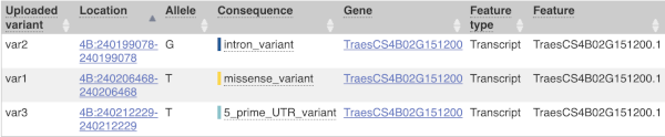
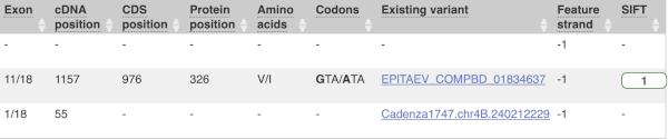
- Use the filters to view only missense variants. The filters are found above the detailed results table in the middle. Select Consequence and is from the drop-down menus. Then type
missense_variantinto the boxe. Add to apply your filter.1 variant is a missense variant. It causes a leucine to arginine (L/R) at position 16 change in the gene OS09G0103500. The SIFT score is 0.01 (Deleterious low confidence). Refere to this link for more information on SIFT (https://sift.bii.a-star.edu.sg/).
Web VEP analysis of variants in Triticum aestivum (wheat)
You have done whole-genome sequencing and variant-calling experiments for Triticum aestivum. You have a VCF file with a small subset of variants from this experiment. Analyse the variants in this file with the VEP tool in Ensembl Plants and determine the following:
-
How many variants were analysed? How many are novel?
-
How many genes and transcripts are affected by variants in this file?
-
Do any of the variants have different consequences for different transcripts?
-
Filter the table to find variants with high impact. How many variants have high impact? Why do you think missense variants are not classified as high impact?
-
Can you export all the results to a VCF file? Compare it to the input VCF file to see what information the VEP adds.
Go to any Ensembl Plants page and click on Tools in the navigation bar at the top of the page. Click on Variant Effect Predictor and change your species to Triticum aestivum by clicking on Change species.
Enter a descriptive name for your VEP job. If you have downloaded the variant file to your local machine, click on Choose file to upload. Alternatively, you can paste the URL for the file into the Or provide file URL: box. Click Run at the bottom of the page. When your job is done, click View reesults.
-
20 variants were analysed, of which 1 is novel.
-
Only 1 gene is affected by variants in this file. The gene has 2 transcripts and both are affected by the variants.
- You can find a list of calculated variant consequences and their impact here.
Yes, the novel variant results in a stop_lost in TraesCS3A02G301400.1 and is a downstream_gene_variant for TraesCS3A02G301400.2.
- Use the filters to view only variants with HIGH impact (you may need to add the column under Show/hide columns at the top of the table if you cannot find it). The filters are found above the detailed results table in the middle. Select Impact and is from the drop-down menus. Then type
HIGHinto the box; this will autocomplete. Click Add.There are 3 variants with high impact and all three are stop altering. Missense variants are not classified as high impact, because they do not always have significant impacts on protein functions. Usually the protein is still produced. In contrast, stop altering variants affect the protein length, and therefore likely affect the protein function.
- At the top right of the table there is an option to download data. Click on VCF for the All option. Open the VCF file you have downloaded in a text editor. You can see that VEP adds annotation in the INFO column of the VCF file.
Command-line VEP analysis of variants in Oryza sativa (rice) via Docker
In the Mapping and variant calling practical session, you produced a VCF file with variant calls for Oryza sativa chromosome 10 using sequencing reads from the 3,000 Rice Genomes Project.
-
Use the command-line VEP tool via Docker to annotate the variants in your VCF file. You can use your own file from the previous module, but it can also be found within the Docker image at
/home/vep/variant_data/SAMEA2569438.chr10.filt.vcf.gz. -
Re-run the command-line VEP tool via Docker to annotate the variants in your VCF including SIFT scores and affected protein domains. Save the output of this query into a separate output file.
-
Use the
filter_VEPtool to find variants that are located within genes in the Disease Resistance Protein (RP) Panther family. -
Use the
filter_VEPtool to find missense variants that have a deleterious SIFT score and are located within genes in the RP Panther family.
- You can run VEP via Docker using the following script:
docker run -t -i -v $HOME/Desktop/VEP/Plants/vep_data:/data csicunam/bioinformatics_iamz:latest \
  vep -i variant_data/SAMEA2569438.chr10.filt.vcf.gz -o /data/output_1.txt --dir /data\
  --cache --cache_version 62 --genomes --species oryza_sativa --force_overwrite --check_existing
Your own script may not look exactly like this and you may employ different flags:
--input_fileor-iAllows you to specify the location of the input file. If your input file is located within your local working directory, don’t forget to specify this by preceding the file name with/data/(this is the equivalent to your local directory).
--output_fileor-oAllows you to specify the name of the output file.
--force_overwriteAllows VEP to overwrite a pre-existing output file with the same name.
--genomesPoints VEP to the Ensembl Genomes (non-vertebrates) server.
--cacheEnables the use of the cache (this can speed up VEP significantly).
--cache_versonAllows you to specify the cache version. This should be used with Ensembl Genomes caches, since their version numbers do not match Ensembl versions. For example, the VEP/Ensembl version may be 115 and the Ensembl Genomes version 62.
--check_existingChecks for the existence of known variants that are co-located with your input variants.
--offlineEnables offline mode (no database connections are made).View the output for exercise 1 here.
- Use the same query as in the previous exercise with 2 additional flags (
--sift band--domains):docker run -t -i -v $HOME/Desktop/VEP/Plants/vep_data:/data csicunam/bioinformatics_iamz:latest \ vep -i variant_data/SAMEA2569438.chr10.filt.vcf.gz -o /data/output_SIFT_and_domains.txt --dir /data\ --cache --cache_version 62 --genomes --species oryza_sativa --check_existing --sift b --domainsThe options are as follows:
--sift bReturns the score and prediction for the SIFT algorithm, which predicts the pathogenicity of missense variants upon protein function.
--domainsAdds the names of the overlapping protein domains to the VEP output.View the output for exercise 2 here.
- The following script uses the
filter_VEPtool to find variants that are located within genes in the RP Panther family:docker run -t -i -v $HOME/Desktop/VEP/Plants/vep_data:/data csicunam/bioinformatics_iamz:latest \ filter_vep -i /data/output_SIFT_and_domains.txt -o /data/output_filtered_e3.txt \ --filter "domains matches PTHR23155"View the output for exercise 3 here.
- The following script uses the
filter_VEPtool to find missense variants that have a deleterious SIFT score and are located within genes in the RP Panther family:docker run -t -i -v $HOME/Desktop/VEP/Plants/vep_data:/data csicunam/bioinformatics_iamz:latest \ filter_vep -i /data/output_SIFT_and_domains.txt -o /data/output_filtered_e4.txt \ --filter "domains matches PTHR23155" --filter "SIFT is deleterious"View the output for exercise 4 here.
Plants comparative genomics
Demo: gene trees and homology predictions
Plants Compara
Gene trees
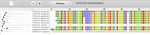
Let’s look at the homologues of Triticum aestivum (wheat) TraesCS3D02G007500. Open Ensembl Plants, search for the gene and go to the Gene tab.
Click on Plant compara: Gene tree, which will display the current gene in the context of a phylogenetic tree used to determine orthologues, paralogues and homoeologues.
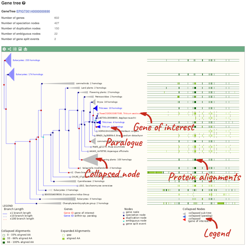
Funnels indicate collapsed nodes. We can expand them by clicking on the node and selecting Expand this sub-tree from the pop-up menu.
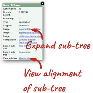
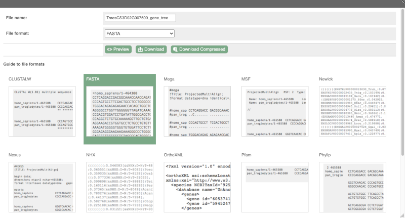
We can also see the protein alignment of the sub-tree by clicking on Wasabi viewer, which will open a pop-up:
You can download the tree in a variety of formats. Click on the download icon ![]() in the bar at the top of the image to get a pop-up where you can choose your format.
in the bar at the top of the image to get a pop-up where you can choose your format.
Homologues
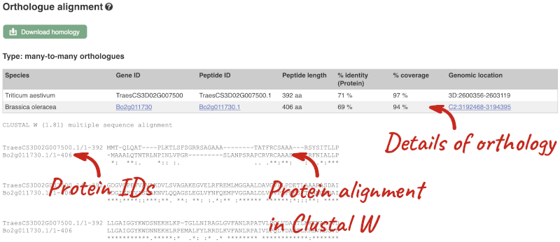
We can look at homologues in the Orthologues, Paralogues and homoeologues pages, which can be accessed from the left-hand menu. If there are no orthologues, paralogues or homoeologues, then the name will be greyed out. Click on Plant compara: Orthologues to see the orthologues available in plants.
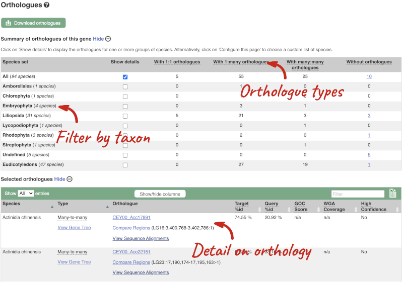
Choose to see only Eudicotyledons orthologues by selecting the box. The table below will now only show details of Eudicotyledons orthologues. Let’s look at Brassica oleracea.
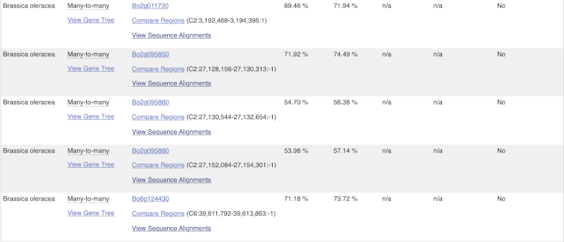
Here we can see there is a many-to-many relationship between the wheat and B. oleracea orthologues. Links from the orthologue allow you to go to alignments of the orthologous proteins and cDNAs. Click on View Sequence Alignments then View Protein Alignment for the first B. oleracea orthologue.
The paralogue page and homoeologue pages are structured in the same way as the orthologue page.
Let’s look at some of the comparative genomics views in the Location tab. Go to the region 1:8000-18000 in Oryza sativa Japonica.
We can look at individual species comparative genomics tracks in this view by clicking on Configure this page.
Select BLASTz/LASTz alignments from the left-hand menu to choose alignments between closely related species. Turn on the alignments for all Oryza species:
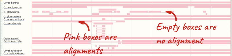
The alignment is greatest between closely related species. We can see that many rice species (such as Oryza barthii) are fully aligned across the region, but other species have a region around 1:10700-12500 where a different chunk is aligned (such as Oryza punctata).
We can also look at the alignment between species or groups of species as text. Click on Alignments (text) in the left hand menu.
Select Select an alignment to open the alignment menu.
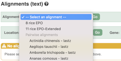
Select Oryza punctata from the alignments list then click Go.
In this case there are eight blocks aligned of different lengths, some of which correspond to the region we saw unaligned in the image. Click on Block 1.
You will see a list of the regions aligned, followed by the sequence alignment. Click on Display full alignment. Exons are shown in red.
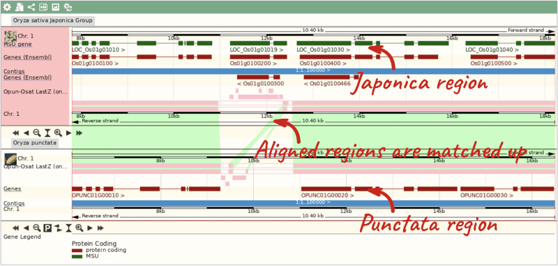
To compare with both contigs visually, go to Region comparison.
To add species to this view, click on the blue Select species or regions button. Choose Oryza punctata again then close the menu.
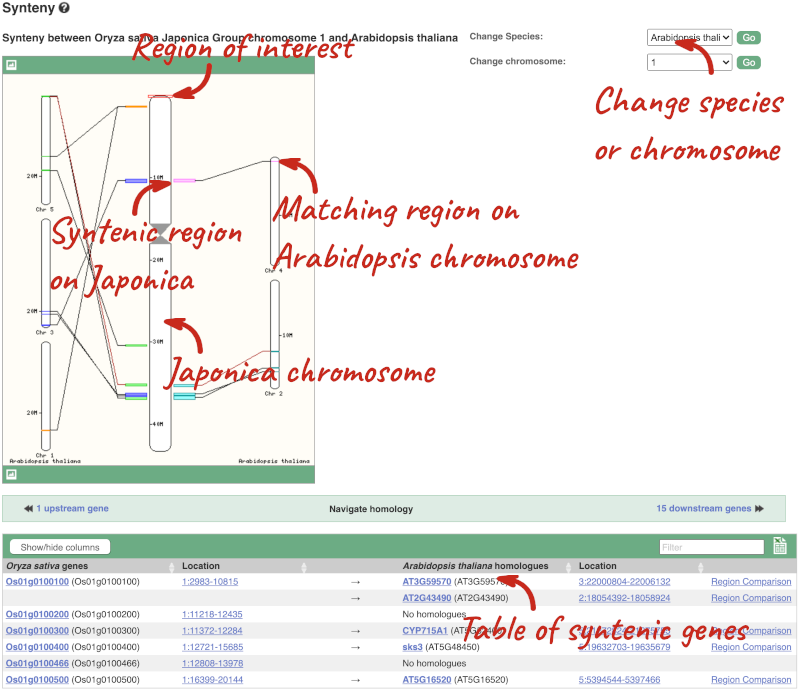
We can view large scale syntenic regions from our chromosome of interest. Click on Synteny in the left hand menu.
Finding orthologues and gene trees of the Arabidopsis thaliana FUM1 gene
The fumarase gene FUM1 in Arabidopsis thaliana encodes a protein with mitochondrial targeting information. Read more in this UniProt entry. Go to Ensembl Plants to answer the following questions:
-
How many orthologues have been identified for this gene?
-
Which orthologue has the highest sequence similarity? Look at the Query%ID and Target%ID.
- Go to Ensembl Plants, select Arabidopsis thaliana from the Favourite genomes section on the homepage. Search for
FUM1. Click on the gene ID AT2G47510. Now click on Plant Compara: Orthologues on the left-hand panel to see all orthologues of this gene. You can find the number of orthologues in the summary information at the top of the page.FUM1 has 166 orthologues in Ensembl Plants.
- Click on the triangles in the table column headers to sort by identity. If you are unsure of what data the column is show, you can mouse-over the headers for a description.
The orthologue with the highest sequence similarity is from Arabidopsis halleri.
Homologues and gene trees for the Triticum aestivum (wheat) RHT1 gene
Go to Ensembl Plants and answer the following questions:
-
How many orthologues are predicted for the Triticum aestivum (wheat) gene RHT1 (gene ID TraesCS4D02G040400) gene in Liliopsida?
-
How much sequence identity does the Secale cereale (rye) protein have to the maize one?
-
Download the alignment in Nexus format.
-
Open the gene tree for the wheat RHT1 gene. What is the gene tree ID?
-
How many speciation and duplication nodes does the phylogeny have?
Go to the Ensembl Plants homepage, select Triticum aestivum from the Species drop-down and search for TraesCS4D02G040400. Click through to the Gene tab. On the Gene tab, click on Plant Compara: Orthologues at the left-hand side of the page to see all the orthologous genes.
- These are the orthologues in the Liliopsida:
- 24 1-to-1
- 9 1-to-many
- 0 many-to-many
- Filter the table by entering
Secale cerealein the filter box on the top right-hand corner of the table.The percentage of identical amino acids in the rye protein (the orthologue) compared with the gene of interest (i.e. wheat RHT1; the target species/gene) is 98.71%. This is known as the Target %ID. The identity of the gene of interest (wheat RHT1) when compared with the orthologue (the rye gene, i.e. the query species/gene) is 97.91% (the query %ID).
Note the differences in the values of the Target and Query % ID reflects the different protein lengths for the genes. -
Click on View Sequence Alignments in the Orthologue column. Select View Protein Alignment from the pop-up menu. Click on the green Download homology button above the table and select Nexus. Click on Download or Download Compressed to save the alignment on your local machine.
- Go to Plant Compara: Gene tree in the left-hand menu. You can find the gene tree ID above the phylogeny.
The gene tree ID is EPlGT00940000163877.
- You can find some summary statistics below the gene ID.
There are 418 speciation nodes and 149 duplication nodes.
Exploring whole-genome alignments for Triticum aestivum (wheat)
Go to Ensembl Plants and answer the following questions:
-
Find the TraesCS2D02G080000 gene in Triticum aestivum (wheat). What is the function for this gene and what are its coordinates?
-
Go to the Location tab. Turn on the LASTZ-net alignment tracks for Arabidopsis thaliana, Zea mays (corn) and Sorghum bicolor (great millet). Are there any regions where you can see gaps in in some of the species alignments?
-
Go to the Region comparison view and compare to A. thaliana. What occurs at this gap in the alignment?
-
Export the Block 2 alignment between T. aestivum and A. thaliana in ClustalW format.
- Go to the Ensembl Plants homepage. Select Triticum aestivum from the Species drop-down, enter
TraesCS2D02G080000in the search box and click Go. Open the Gene tab.The gene description is as follows: Ascorbate peroxidase, ROS homeostasis, Chloroplast protection, Carbohydrate metabolism, Plant architecture, Fertility maintenance. This was projected from Oryza sativa (Os07g0694700).
- Go the Location tab in the top left-hand corner. Click on CConfigure this page in the side menu. Open Comparative genomics: BLASTz/LASTz alignments in the pop-up menu. Turn on the tracks for Arabidopsis thaliana, Zea mays (corn) and Sorghum bicolor (great millet) in the Normal style. Save and close the pop-up menu
There is alignment across most of the coding regions, with some gaps occurring in all 3 species. These gaps map with the intronic regions of the T. aestivum gene.
- Click on Comparative Genomics: Region Comparison in the left-hand menu. Go to the Select species or regions button and add A. thaliana. Save and close the menu.
The gap in the alignment translates to the intronic regions of the T. aestivum gene.
- Go to Comparative Genomics: Alignments (text) and select A. thaliana from the Alignment drop-down. Click on the green Download alignment button and select ClustalW. Download the file to your local machine either in a compressed format, or as it is by clicking the green Download button above the file format preview.
Orthologues, paralogues and gene trees for the maize Zm00001d015746 gene
How many orthologues are predicted for the maize Zm00001d015746 gene in Liliopsida?
How much sequence identity does the Sorghum bicolor protein have to the maize one? Click on the Alignment link next to the Ensembl identifier column to view a protein alignment in Clustal format.
Go to plants.ensembl.org, choose Zea mays and search for Zm00001d015746. Click through to the Gene tab view.
On the gene tab, click on Orthologues at the left side of the page to see all the orthologous genes.
These are the orthologues in the Liliopsida:
- 20 1-to-1
- Seven 1-to-many
- Two many-to-many
The percentage of identical amino acids in the sorghum protein (the orthologue) compared with the gene of interest. i.e. maize Zm00001d015746 (the target species/gene) is 82.07%. This is known as the Target %ID. The identity of the gene of interest (maize GRMZM2G144081) when compared with the orthologue (the sorghum gene, the query species/gene) is 81.69% (the query %ID).
Note the differences in the values of the Target and Query % ID reflects the different protein lengths for the genes.
Finding orthologous genes for disease resistance gene in Coffea canephora (coffee)
Resistance to the leaf rust delivered by SH3 factor(s) is well-grounded as specially durable. in 2023, Paula Cristina da Silva Angelo et al (https://doi.org/10.1016/j.pmpp.2023.102111) reported that the Arabidopsis thaliana gene AT1G50180 is an important gene in the SH3 locus conferring diseae resistance.
Search Ensembl Plants for the gene AT1G50180 in Arabidopsis thaliana.
-
From the gene tab, go to the Arabidopsis thaliana AT1G50180 gene Orthologues page under Plant Compara.
-
Reduce the orthologues table to look only at Coffea canephora (coffee) orthologues. How many results can you see?
-
Download the cDNA alignment in ClustalW format for the alignment between the Arabidopsis thaliana AT1G50180 gene and the Coffea canephora GSCOC_T00030728001 gene.
Go to Ensembl Plants. Select Arabidopsis thaliana from the drop-down box and type in AT1G50180. Click Go and click on the gene ID AT1G50180.
-
Go to Plant Compara: Orthologues on the left-hand panel.
- Filter for Coffea canephora using the filter option in the top right hand corner of the table.
Coffee has 25 many-to-many orthologues.
- Click on View Sequence Alignments then cDNA (found in the 3rd column below the gene identifier) for the GSCOC_T00030728001 gene. This takes us to the Orthologue Alignment page.
Click on Download Homology to download the alignment in ClustalW format
Finding orthologous genes for a root transporter in Oryza sativa Japonica (rice)
Search Ensembl Plants for the gene Lsi1 in Oryza sativa Japonica Group (rice). This gene is known to code for an aquaporin transporter that facilitates the uptake of silicon and arsenic through the roots. Silicon concentration is highest in grass species, and is associated with defence.
-
From the gene tab, go to the Orthologues page under Plant Compara. Which plant group has the highest number of 1-to-1 orthologues? Is it the same group that has the highest number of 1-to-many orthologues?
-
Reduce the orthologues table to look only at Triticum aestivum (wheat) orthologues. Why are there three results for a 1-to-1 orthologue?
-
Click on the Compare regions link for chromosome 6B region in wheat to go to the Location tab. Scroll to the bottom image. How do the gene models compare between the species? Do they have the same number of exons?
-
Click back to the Gene tab and click on the Gene gain/loss tree page. Which species has the highest number of members of this gene family? Is it a grass? Can you change the view to see a radial tree?
Go to Ensembl Plants. Look for the main search box highlighted in green. Select Oryza sativa Japonica Group from the drop-down box and type in Lsi1. Click Go and click on the gene ID Os02g0745100.
- Go to Plant Compara: Orthologues on the left-hand panel.
Liliopsida has 24 1-to-1 orthologues, the only group with 1-to-1 orthologues. This group is synonymous with Monocotyledon, so the group that contains the grasses. Eudicotyledons has the highest number of 1-to-many orthologues, indicating that this gene has been duplicated in the eudicots.
- Use the search box in the top right-hand corner of the Selected orthologues table and enter
Triticum aestivum, the table should automatically filter.There are 3 results, one for each component (A,B,D). Note that these are considered 1-to-1 orthologues, rather than 1-to-many. This is because these genes arose in wheat by hybridisation (allopolyploidy), rather than duplication (autopolyploidy).
- Click on Compare regions (found in the 3rd column below the gene identifier) from the 2nd result for component 6B. This takes us to the Location tab. Scroll down to the bottom of the page.
Both genes have 5 exons and the same structure. This looks unusual because the gene in rice is on the forward strand, while the gene in wheat is on the reverse strand. This is reflected in the crossing green links between the pink alignment blocks.
- Click on the Gene tab at the top of the page and click on Gene gain/loss tree in the left-hand panel.
Significant expansions are shown with red branches, and the number of genes in the family shown in the count next to the image and species name. We can see that Echinochloa crus-galli (Cockspur grass) has 25 members in this group.
We can change the tree to radial view by clicking on the icon with two arrows at the top left of the image.