Ensembl Homepage

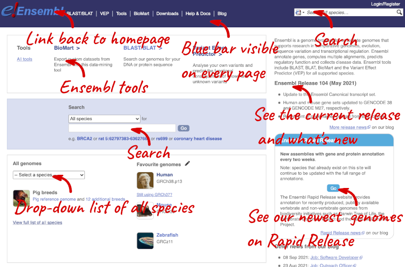
The front page of Ensembl is found at ensembl.org. It contains lots of information and links to help you navigate Ensembl:

At the top left you can see the current release number and what has come out in this release. To access old releases, scroll to the bottom of the page and click on View in archive site.

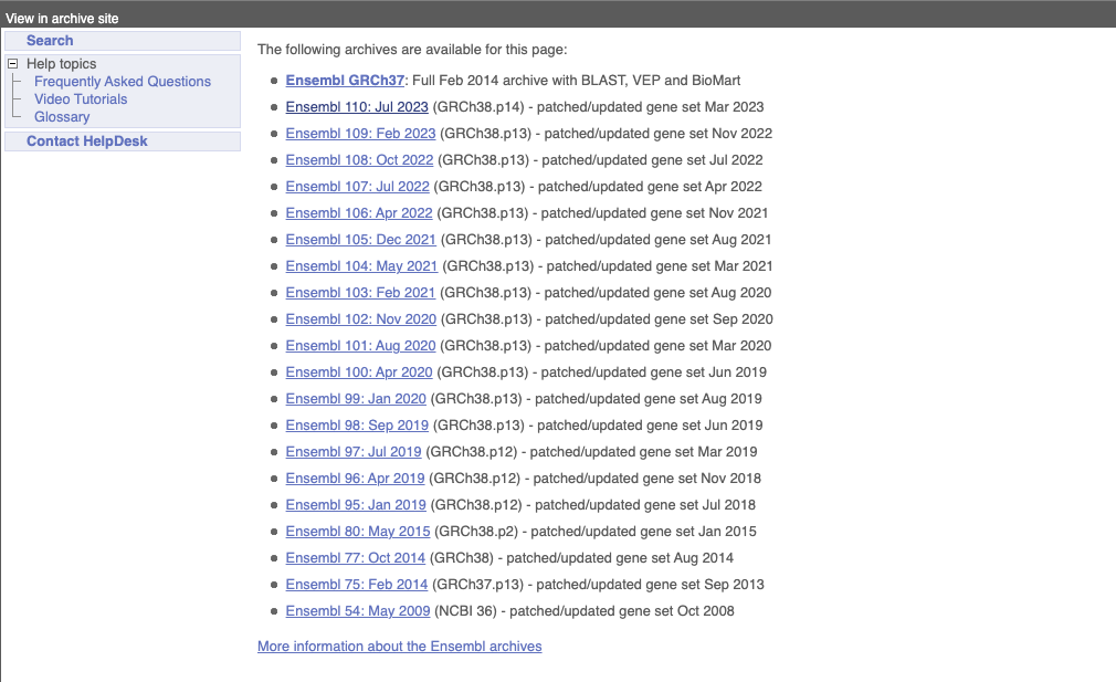
Click on the links to go to the archives. Alternatively, you can jump quickly to the correct release by putting it into the URL, for example e98.ensembl.org jumps to release 98.

Click on View full list of all species.

Click on the common name of your species of interest to go to the species homepage. We’ll click on Human.

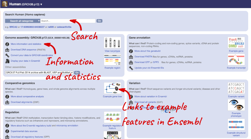
Here you can see links to example pages and to download flatfiles. To find out more about the genome assembly and genebuild, click on More information and statistics.

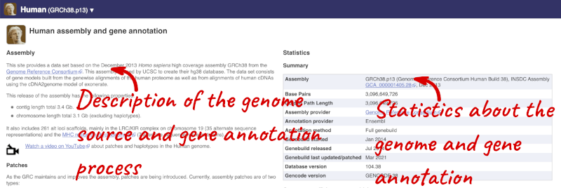
Here you’ll find a detailed description of how to the genome was produced and links to the original source. You will also see details of how the genes were annotated.

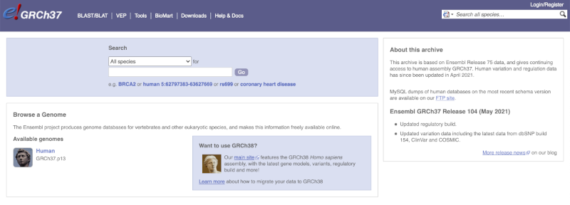
The current genome assembly for human is GRCh38. If you want to see the previous assembly, GRCh37, visit our dedicated site grch37.ensembl.org.

Region in detail view

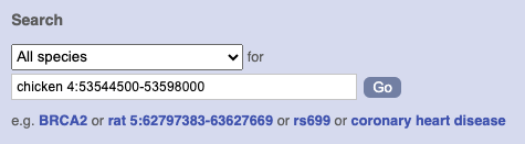
Start at the Ensembl front page, ensembl.org. You can search for a region by typing it into a search box, but you have to specify the species.

To bypass the text search, you need to input your region coordinates in the correct format, which is chromosome, colon, start coordinate, dash, end coordinate, with no spaces for example: human 4:122868000-122946000. Type (or copy and paste) these coordinates into either search box.

or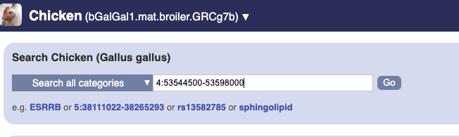

Press Enter or click Go to jump directly to the Region in detail Page.

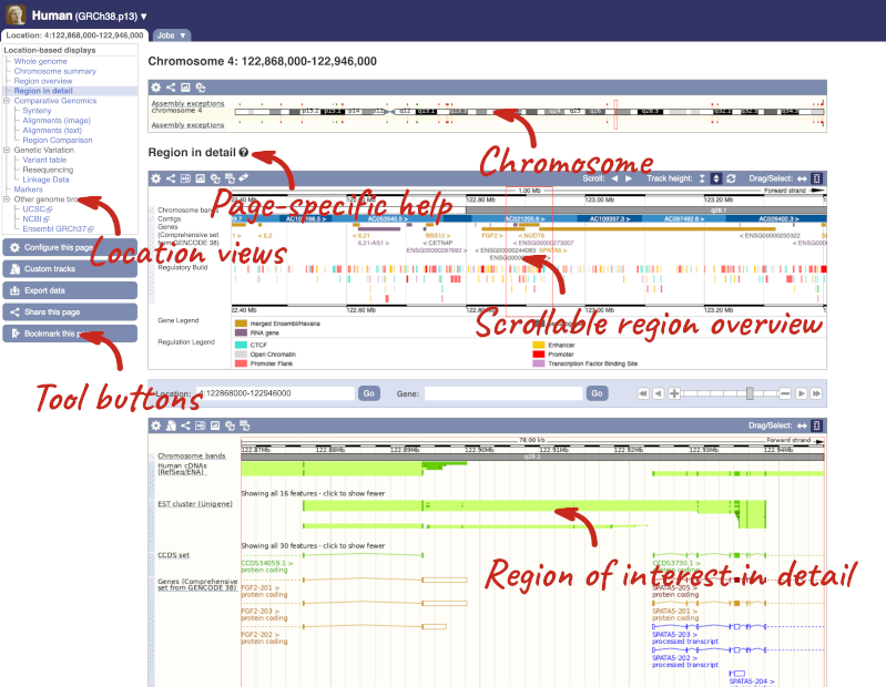
Click on the button to view page-specific help. The help pages provide text, labelled images and, in some cases, help videos to describe what you can see on the page and how to interact with it.

The Region in detail page is made up of three images, let’s look at each one in detail.

1. The first image shows the chromosome:

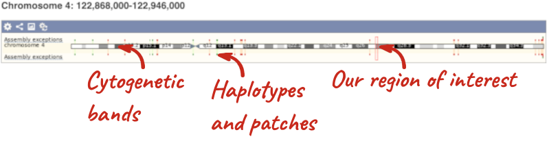
The region we’re looking at is highlighted on the chromosome. You can jump to a different region by dragging out a box in this image. Drag out a box on the chromosome, a pop-up menu will appear.

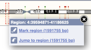
If you wanted to move to the region, you could click on Jump to region (### bp). If you wanted to highlight it, click on Mark region (###bp). For now, we’ll close the pop-up by clicking on the X on the corner.

1. The second image shows a 1Mb region around our selected region. This is always 1Mb in human, but the fixed size of this view varies between species. This view allows you to scroll back and forth along the chromosome.

You can also drag out and jump to or mark a region.

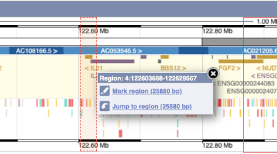
Click on the X to close the pop-up menu.

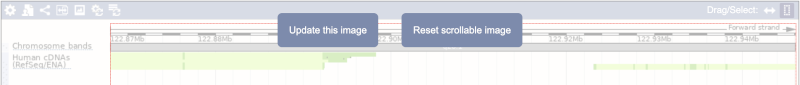
Click on the Drag/Select button to change the action of your mouse click. Now you can scroll along the chromosome by clicking and dragging within the image. As you do this you’ll see the image below grey out and two blue buttons appear. Clicking on Update this image would jump the lower image to the region central to the scrollable image. We want to go back to where we started, so we’ll click on Reset scrollable image.

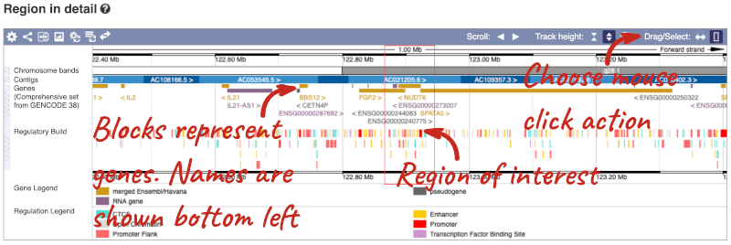
1. The third image is a detailed, configurable view of the region.

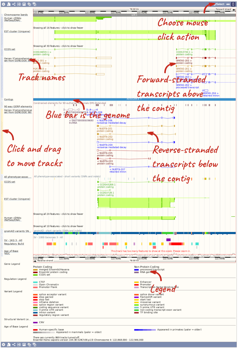
Here you can see various tracks, which is what we call a data type that you can plot against the genome. Some tracks, such as the transcripts, can be on the forward or reverse strand. Forward stranded features are shown above the blue contig track that runs across the middle of the image, with reverse stranded features below the contig. Other tracks, such as variants, regulatory features or conserved regions, refer to both strands of the genome, and these are shown by default at the very top or very bottom of the view.

You can use click and drag to either navigate around the region or highlight regions of interest, Click on the Drag/Select option at the top or bottom right to switch mouse action. On Drag, you can click and drag left or right to move along the genome, the page will reload when you drop the mouse button. On Select you can drag out a box to highlight or zoom in on a region of interest.

With the tool set to Select, drag out a box around an exon and choose Mark region.

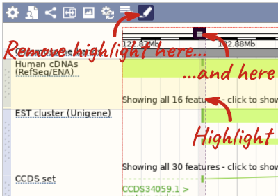
The highlight will remain in place if you zoom in and out or move around the region. This allows you to keep track of regions or features of interest.

We can edit what we see on this page by clicking on the blue Configure this page menu at the left.

This will open a menu that allows you to change the image.

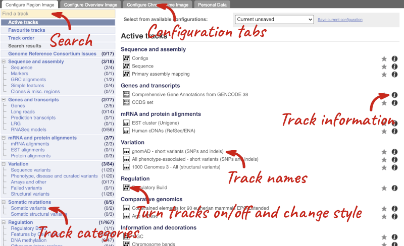
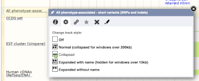
There are thousands of possible tracks that you can add. When you launch the view, you will see all the tracks that are currently turned on with their names on the left and an info icon on the right, which you can click on to expand the description of the track. Turn them on or off, or change the track style by clicking on the box next to the name. More details about the different track styles are in this FAQ: http://www.ensembl.org/Help/Faq?id=335.

You can find more tracks to add by either exploring the categories on the left, or using the Find a track option at the top left. Type in a word or phrase to find tracks with it in the track name or description.

Let’s add some tracks to this image. Add:

• Proteins (mammal) from UniProt – Labels
• 1000 Genomes - All - short variants (SNPs and indels) – Normal

Now click on the tick in the top left hand to save and close the menu. Alternatively, click anywhere outside of the menu. We can now see the tracks in the image. The proteins track is stranded, so you will see two tracks, one above and one below the contig, representing the proteins mapped to the forward and reverse strands respectively. The variants track is not stranded, so is found near the bottom of the image.

If the track is not giving you can information you need, you can easily change the way the tracks appear by hovering over the track name then the cog wheel to open a menu. To make it easier to compare information between tracks, such as spotting overlaps, you can move tracks around by clicking and dragging on the bar to the left of the track name.

Now that you’ve got the view how you want it, you might like to show something you’ve found to a colleague or collaborator. Click on the Share this page button to generate a link. Email the link to someone else, so that they can see the same view as you, including all the tracks you’ve added. These links contain the Ensembl release number, so if a new release or even assembly comes out, your link will just take you to the archive site for the release it was made on.

To return this to the default view, go to Configure this page and select Reset configuration at the bottom of the menu.

Genes and transcripts

You can find out lots of information about Ensembl genes and transcripts using the browser. If you’re already looking at a region view, you can click on any transcript and a pop-up menu will appear, allowing you to jump directly to that gene or transcript.

Alternatively, you can find a gene by searching for it. You can search for gene names or identifiers, and also phenotypes or functions that might be associated with the genes.

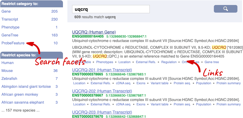
We’re going to look at the human UQCRQ gene. From ensembl.org, type UQCRQ into the search bar and click the Go button. You will get a list of hits with the human gene at the top.

Where you search for something without specifying the species, or where the ID is not restricted to a single species, the most popular species will appear first, in this case, human, mouse and zebrafish appear first. You can restrict your query to species or features of interest using the options on the left.

The gene tab

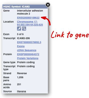
Click on the gene name or Ensembl ID. The Gene tab should open:

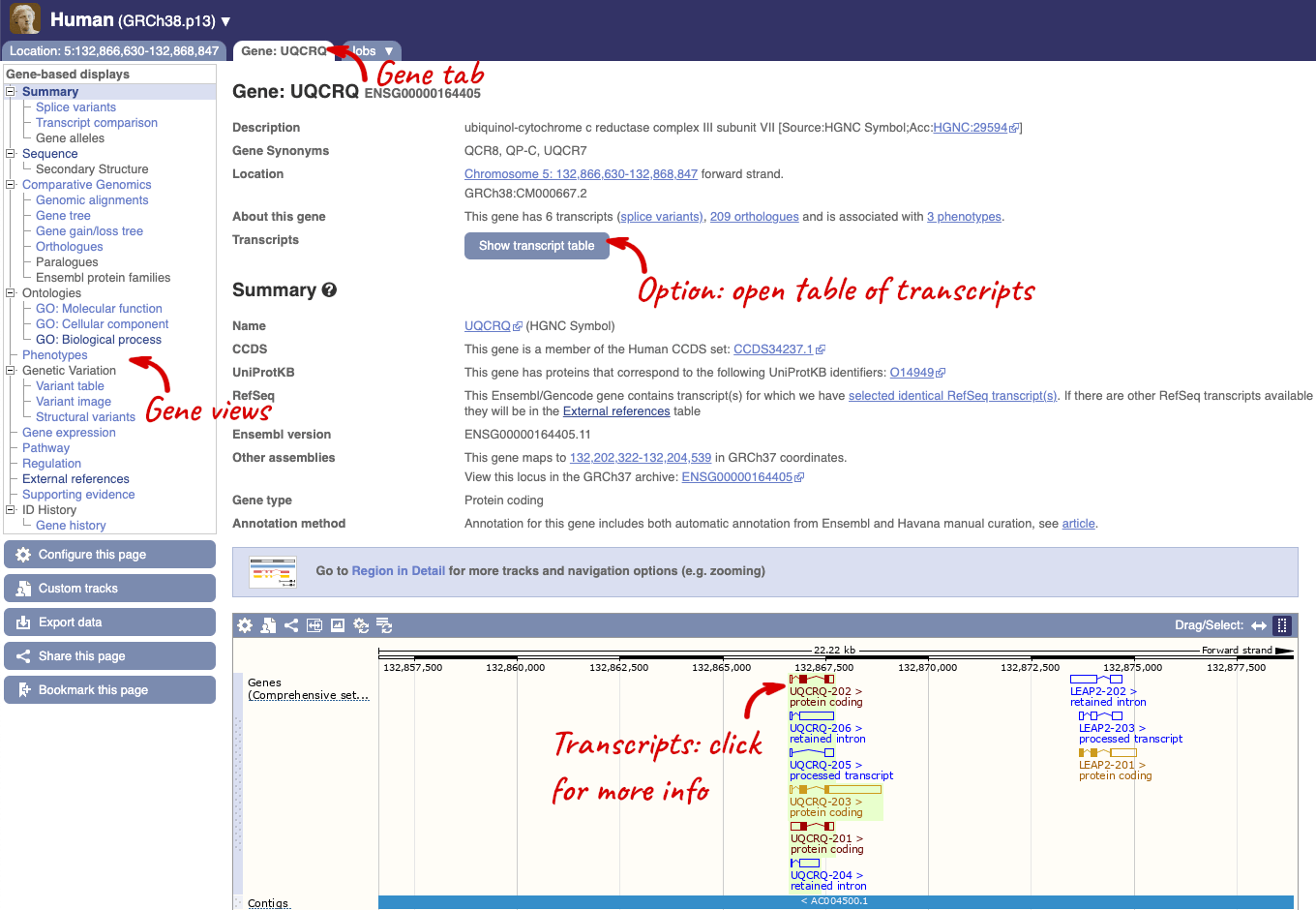
This page summarises the gene, including its location, name and equivalents in other databases. At the bottom of the page, a graphic shows a region view with the transcripts. We can see exons shown as blocks with introns as lines linking them together. Coding exons are filled, whereas non-coding exons are empty. We can also see the overlapping and neighbouring genes and other genomic features.

There are different tabs for different types of features, such as genes, transcripts or variants. These appear side-by-side across the blue bar, allowing you to jump back and forth between features of interest. Each tab has its own navigation column down the left hand side of the page, listing all the things you can see for this feature.

Let’s walk through this menu for the gene tab. How can we view the genomic sequence? Click Sequence at the left of the page.

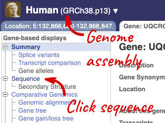
The sequence is shown in FASTA format. The FASTA header contains the genome assembly, chromosome, coordinates and strand (1 or -1) – this gene is on the positive strand.

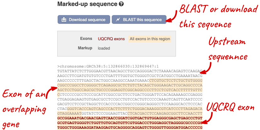
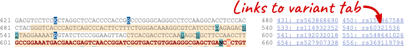
Exons are highlighted within the genomic sequence, both exons of our gene of interest and any neighbouring or overlapping gene. By default, 600 bases are shown up and downstream of the gene. We can make changes to how this sequence appears with the blue Configure this page button found at the left. This allows us to change the flanking regions, add variants, add line numbering and more. Click on it now.

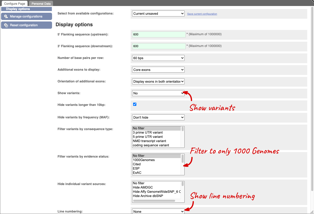
Once you have selected changes (in this example, Show variants, 1000 Genomes variants and Line numbering) click at the top right.

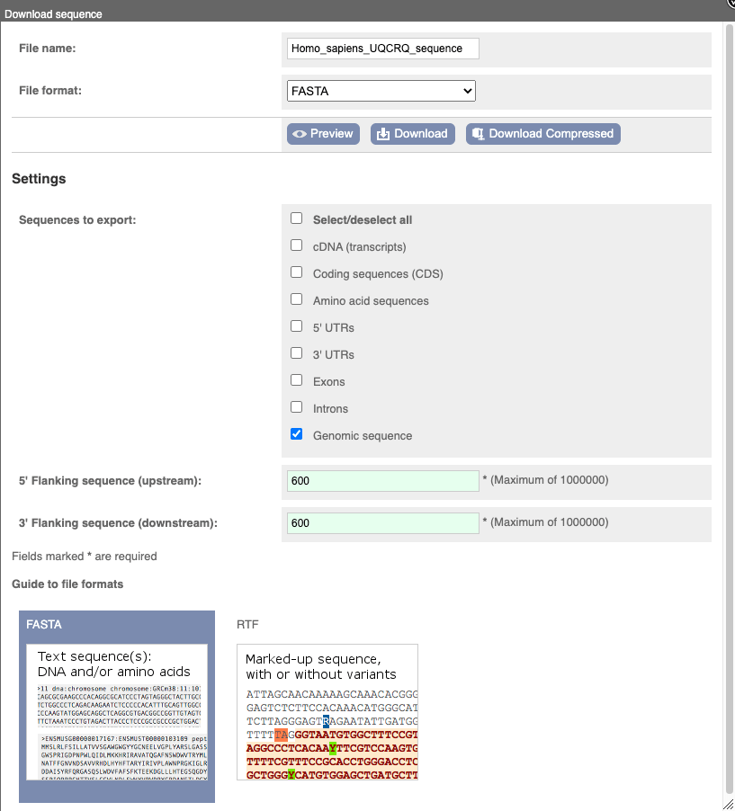
You can download this sequence by clicking in the Download sequence button above the sequence:

This will open a dialogue box that allows you to pick between plain FASTA sequence, or sequence in RTF, which includes all the coloured annotations and can be opened in a word processor. If you want run a sequence analysis tool, download as FASTA sequence, whereas if you want to analyse the sequence visually, RTF is best for this. This button is available for all sequence views.

To find out what the protein does, have a look at GO terms from the Gene Ontology consortium. There are three pages of GO terms, representing the three divisions in GO: Biological process (what the protein does), Cellular component (where the protein is) and Molecular function (how it does it). Click on GO: Biological process to see an example of the GO pages.

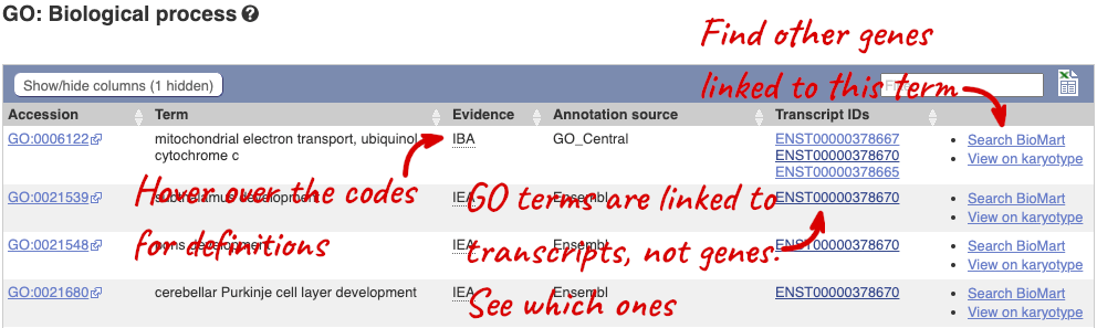
Here you can see the functions that have been associated with the gene. There are three-letter codes that indicate how the association was made, as well as links to the specific transcript they are linked to.

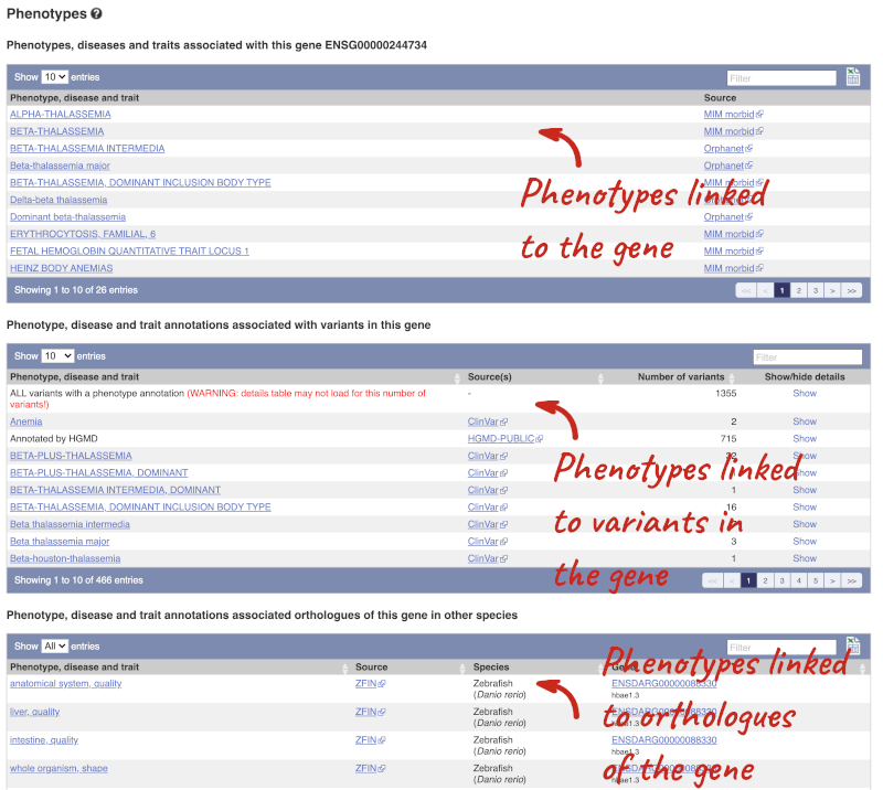
You can also see the phenotypes associated with a gene. Click on Phenotype in the left hand menu.

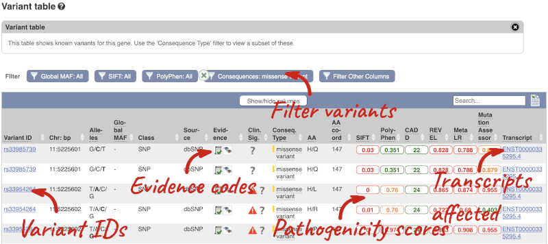
To view all the sequence variants in table form, click the Variant table link at the left of the gene tab.

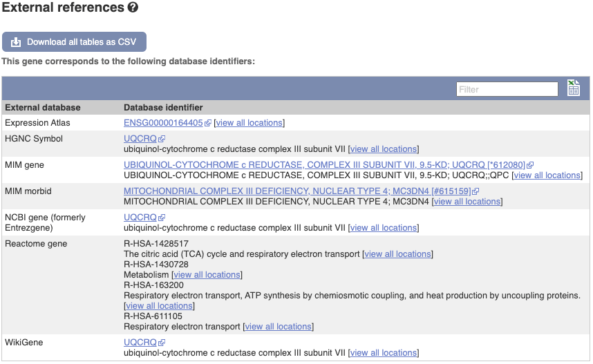
We also have links out to other databases which have information about our genes and may focus on other topics that we don’t cover, like Gene Expression Atlas or OMIM. Go up the left-hand menu to External references:

The transcript tab

We’re now going to explore the different transcripts of UQCRQ. Click on Show transcript table at the top.

Here we can see a list of all the transcripts of UQCRQ with their identifiers, lengths, biotypes and flags to help you decide which ones to look at.

If we were to only choose one transcript to analyse, we would choose UQCRQ-203 because it is the MANE Select and Ensembl Canonical. This means it is both 100% identical to the RefSeq transcript NM_014402.5 and both Ensembl and NCBI agree that it is the most biologically important transcript.

Click on the ID, ENST00000378670.8.

You are now in the Transcript tab for UQCRQ-203. We can still see the gene tab so we can easily jump back. The left hand navigation column provides several options for the transcript UQCRQ-203 - many of these are similar to the options you see in the gene tab, but not all of them. If you can’t find the thing you’re looking for, often the solution is to switch tabs.

Click on the Exons link. This page is useful for designing RT-PCR primers because you can see the sequences of the different exons and their lengths.

You may want to change the display (for example, to show more flanking sequence, or to show full introns). In order to do so click on Configure this page and change the display options accordingly.

Now click on the cDNA link to see the spliced transcript sequence with the amino acid sequence. This page is useful for mapping between the RNA and protein sequences, particularly genetic variants.

UnTranslated Regions (UTRs) are highlighted in dark yellow, codons are highlighted in light yellow, and exon sequence is shown in black or blue letters to show exon divides. Sequence variants are represented by highlighted nucleotides and clickable IUPAC codes are above the sequence.

Next, follow the General identifiers link at the left. Just like the External References page in the gene tab, this page shows links out to other databases such as RefSeq, UniProtKB, PDBe and others, this time linked to the transcript or protein product, rather than the gene.

1. In Ensembl, find the human MYH9 (myosin, heavy chain 9, non-muscle) gene and open the Gene tab.
   • On which chromosome and which strand of the genome is this gene located?
   • How many transcripts (splice variants) are there and how many are protein coding?
   • What is the longest protein-coding transcript, and how long is the protein it encodes?
   • Which transcript would you take forward for further study?

2. Click on Phenotypes at the left side of the page. Are there any diseases associated with this gene, according to Mendelian Inheritance in Man (MIM)?

3. What are some functions of MYH9 according to the Gene Ontology (GO) consortium? Have a look at the GO: Biological process pages for this gene.

4. In the transcript table, click on the transcript ID for MYH9-201, and go to the Transcript tab.
   • How many exons does it have?
   • Are any of the exons completely or partially untranslated?
   • Is there an associated sequence in UniProtKB/Swiss-Prot? Have a look at the General identifiers for this transcript.
5. Are there microarray (oligo) probes that can be used to monitor ENST00000216181 expression?

Phenylketonuria is a genetic disorder caused by an inability to metabolise phenylalanine in any body tissue. This results in an accumulation of phenylalanine causing seizures and intellectual disability.

(a) Search for phenylketonuria from the Ensembl homepage and narrow down your search to only genes. What gene is associated with this disorder?

(b) How many protein coding transcripts does this gene have? View all of these in the transcript comparison view.

(c) What is the MIM gene identifier for this gene?

(d) Go to the MANE Select transcript and look at its 3D structure. In the model 2pah, how many protein molecules can you see?

Go to Ensembl.

1. Go to the region from 32,264,000 to 32,492,000 bp on human chromosome 13. On which cytogenetic band is this region located? How many contigs make up this portion of the assembly (contigs are contiguous stretches of DNA sequence that have been assembled solely based on direct sequencing information)?

2. Zoom in on the BRCA2 gene.

3. Configure this page to turn on the LTR (repeat) track in this view. What tool was used to annotate the LTRs according to the track information? How many LTRs can you see within the BRCA2 gene? Do any overlap exons?

4. Create a Share link for this display. Email it to your neighbour. Open the link they sent you and compare. If there are differences, can you work out why?

5. Export the genomic sequence of the region you are looking at in FASTA format.

6. Turn off all tracks you added to the Region in detail page.

We’re going to look for regulatory features in the region of a gene and investigate their activity in different cell types. We’ll start by searching for the gene KPNA2 and jumping to the Location tab. Scroll down to the Region in detail view and zoom out a little to see the gene as well as its flanking regions.

The Regulatory Build track is shown by default.

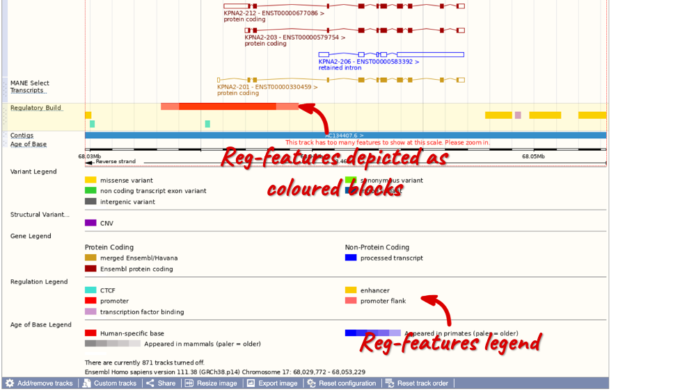
In this region we can see a number of regulatory features, including a red promoter with light red promoter flanks, cyan CTCF binding sites, yellow enhancers and lilac transcription factor (TF) binding sites (don’t worry if you have zoomed out further or not as far and can see more/less). Refer to the legend at the bottom of the view to see what each of the colours mean.

You can also click on the individual regulatory features to learn more. Click on the red promoter to open a pop-up menu.

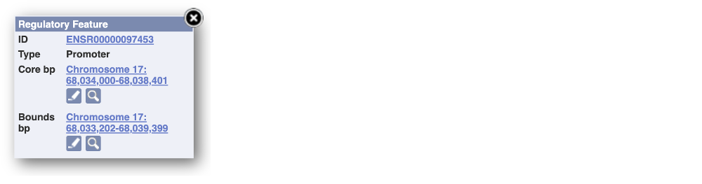
Click on the stable ID, ENSR00000097453, to jump to the Regulation tab.

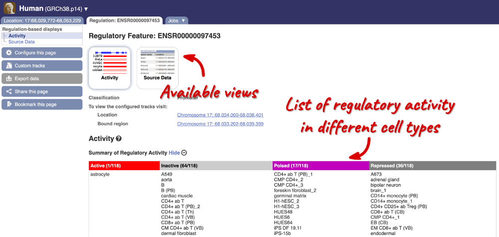
Here, you can find a summary of the activity of the promoter in the different cell types. Scroll down to Summary of Regulatory Aactivity to find out in which cells the promoter is active (the feature displays an active epigenetic signature, which can include evidence of open chromatin), inactive (the region bears no epigenetic modifications from the ones included in the Regulatory Build), poised (the feature displays a epigenetic signature with the potential to be activated) or repressed (the feature is epigenetically suppressed). We can see that this promoter is active in one out of the 118 cell types currently in Ensembl.

Let’s switch back to the Location tab to explore the different regulation tracks that are available. Click on Configure this page and in the pop-up window under the Regulation section, click on Other regulatory regions and enable the Fantom 5, TarBase and Motif features tracks. Close the pop-up window.

The Fantom 5 track displays transcription start site (TSS) and enhancer predictions from the FANTOM5 project.

The TarBase track displays experimentally verified miRNA targets from TarBase.

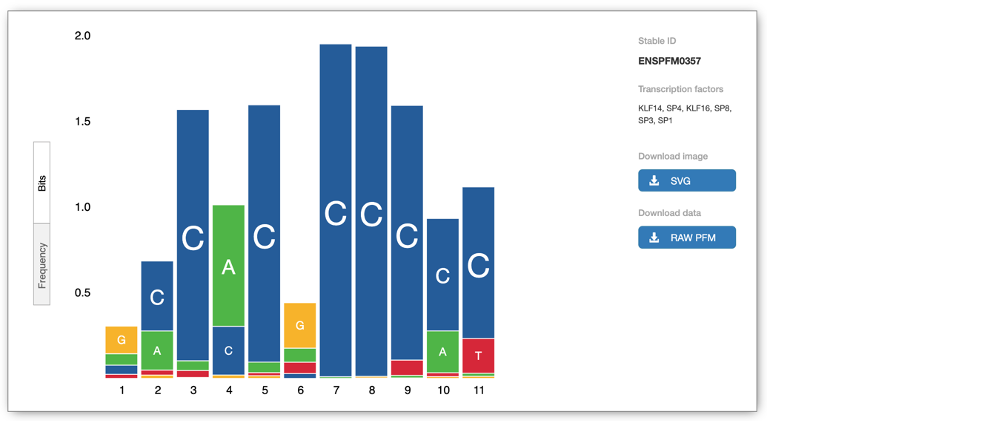
The Motif features track indicates the positions of transcription factor binding motifs (TFBMs) in black lines/blocks. You can click on individual features to find out more information about the TFBM, including a list of TFs binding at this site and, if available, in which cells the TFBM was experimentally verified in. You can also view the Binding matrix** by clicking on the matrix ID. This opens a pop-up window which displays the binding matrix used and a binding score representing how well a particular site matches the binding matrix.

We can explore more detailed data by adding further Regulation tracks. Click on the Configure this page button on the left-hand side.

In the pop-up window, go to Regulation and click on Features by Cell/Tissue to view the detailed activity of the regulatory feature by cell type.

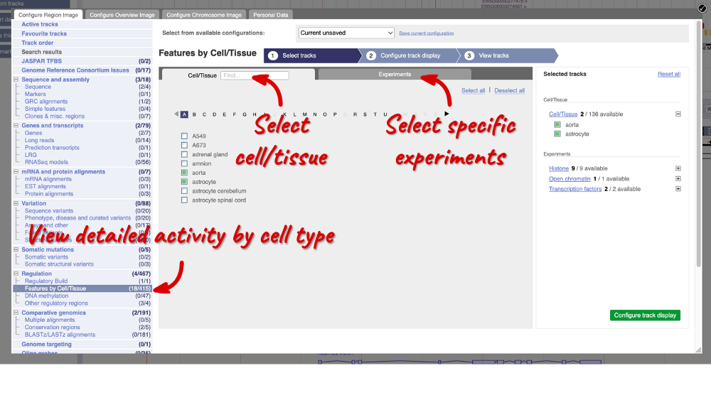
We can add cells by clicking on them. Find them using the search or the alphabet ribbon. Let’s add a cell type where the promoter is inactive, aorta, and one where it’s active astrocytes. Once you’ve selected the cells, they will appear in the menu on the right, where you can easily view the list by clicking on the + icon and de-select them.

To choose the experiments to see data on, click on the Experiments tab at the top of the menu. You can navigate this the same as the Cell/Tissue tab, except that you have to choose between Histone, Open Chromatin and Transcription factors. Let’s Select all in all categories.

When you’ve chosen your experiments and cells, you can click on the green Configure track display button in the bottom right-hand corner.

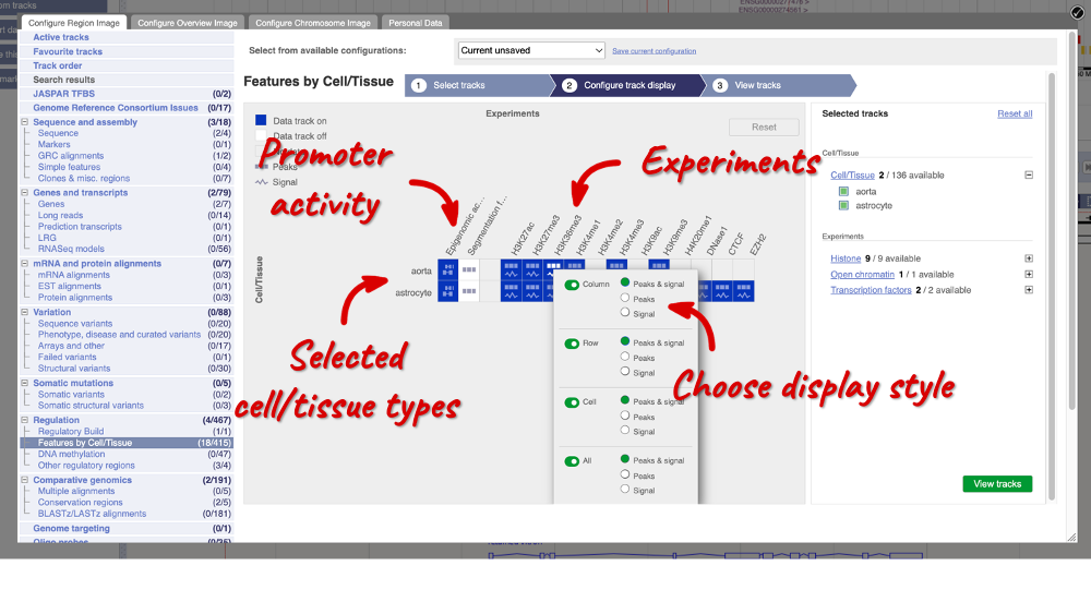
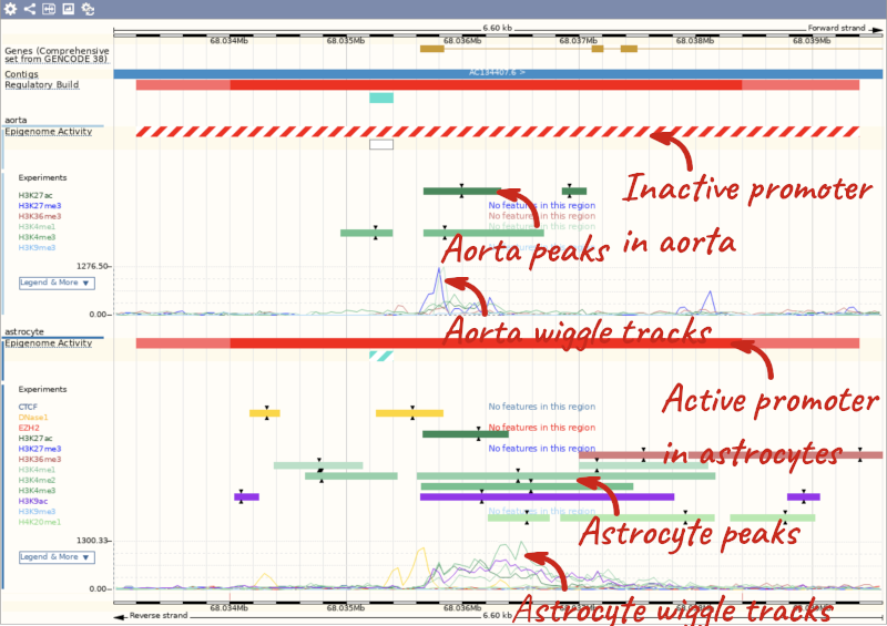
Now we can see the active feature in astrocytes compared to the inactive feature in aorta.

1. Find the Location tab (Region in detail view) for the region between the genes INSIG1 and BLACE. Are there any predicted enhancers in this region?

2. Go to the Regulation tab for the enhancer ENSR00001133586. How many cell types is this enhancer active in? Are there any cell types where its activity is repressed?

3. Switch to the Location tab. Take a look at the histone modifications across this enhancer in neutro myelocyte cells, where this enhancer is active, compared to neutrophil (CB) cells, where it is poised. What differences can you observe?

4. Are there any verified transcription factor binding motifs in this enhancer? In what cells?

1. Search for the regulatory feature ENSR00000262400. What type of feature is this? What is its genomic location?

2. Which cell types is this feature inactive and/or repressed in? View the supporting evidence for the repressed cell type. What project was the repressed cell type studied in?

3. Why do so many cells have this feature listed as NA on the Activity display?

Demo: Upload small files

We have some patients that present with microcephaly and developmental delay. They all have large scale deletions on chromosome five:

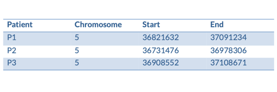
We can turn them into a BED file and view them in the genome browser:

chr5 36821632 37091234 P1
chr5 36731476 36978306 P2
chr5 36908552 37108671 P3

You can add data from a Region in Detail page by clicking on the Custom tracks button at the left. Alternatively, go to a species homepage and click on Display your data in Ensembl.

A menu will appear:

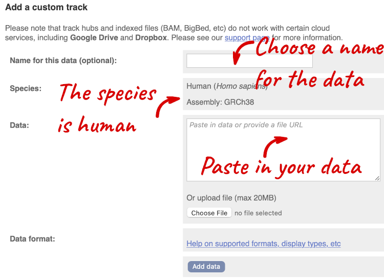
The interface detects file types if you upload or attach a file. When you paste in your data, it can’t do this so we have to tell it what our file type is. It will give you an option where you can select BED.

Click Add data.

You should get to a dialogue box telling you your upload has been successful.

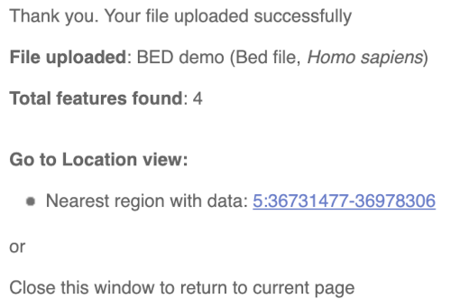
Click on the genomic coordinates link to go to the nearest region with data.

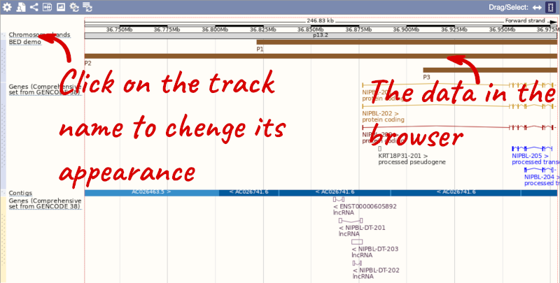
To have a look at the file, click on Custom tracks.

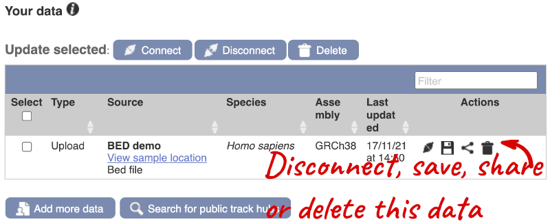
If you’ve got an Ensembl account, you can save this data to your account. Accounts are free to set up and allow you to save configurations and data, and share with groups.

Demo: Attach URLs of large files

Larger files, such as BAM files generated by NGS, need to be attached by URL. I’ve put a BAM file of human chromosome 20 RNASeq data online at: http://ftp.ebi.ac.uk/pub/databases/ensembl/training/emily_BAM/

Let’s take a look at the folder.

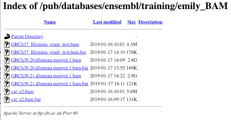
Here you can see a number of BAM files (.bam) with corresponding index files (.bam.bai). We’re interested in the files GRCh38.20.illumina.merged.1.bam and GRCh38.20.illumina.merged.1.bam.bai. These files are the BAM file and the index file respectively. When attaching a BAM file to Ensembl, there must be an index file in the same folder.

To attach the file, click on Custom tracks, then click on Add more data to add a new track.

We get to the same dialogue box as before. This time we’ll name our data Illumina reads.

Paste in the URL of the BAM file itself (http://ftp.ebi.ac.uk/pub/databases/ensembl/training/emily_BAM/GRCh38.20.illumina.merged.1.bam).

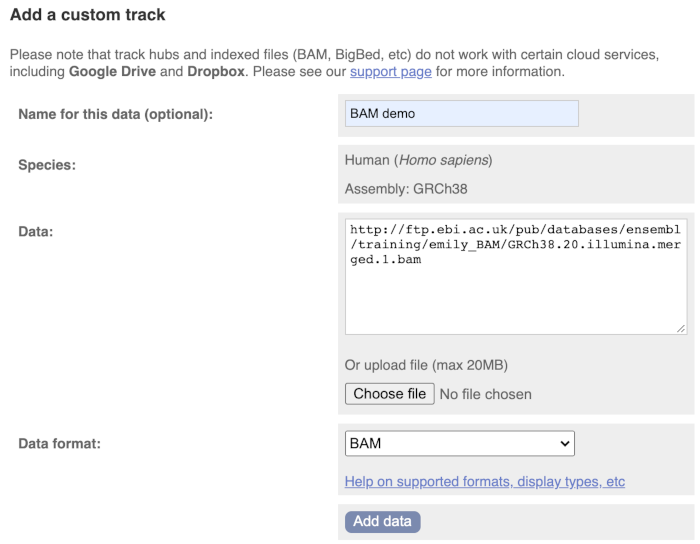
Since this is a file, the interface is able to detect the “.BAM” file extension, so automatically labels the format as BAM. Click on Add data and close the menu.

To see this data, jump to a region on chromosome 20. Let’s go to the region of the CDH22 gene. Search for the gene and click on the location.

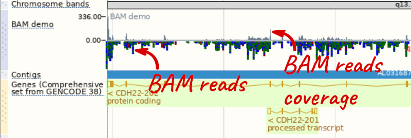
We can zoom in to see the sequence itself. Drag out boxes in the view to zoom in, until you see a view like this. Alternatively, jump to location 20:46241000-46241030.

Demo: Track hub registry

Our regulatory data incorporates data from sources such as ENCODE, Blueprint, and Roadmap Epigenomics. To see the data directly from these sources, you can add track hubs.

You can search for track hubs to add in different ways:

• Search for track hubs in the Track Hub Registry and choose to add them to your genome browser of choice.
• Search the track hub registry using the Track Hub Registry interface in Ensembl (there is a link from the homepage).

We will now add the track hub containing data from the Blueprint project.

You can add track hubs to view in Ensembl directly via the Track Hub Registry. Go to the Track Hub Registry homepage and search for blueprint.

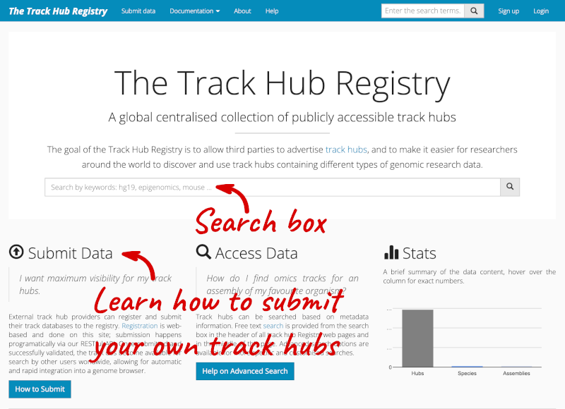
There are two results for the Blueprint Hub, one for adding the track hub to GRCh37 and one for adding it to GRCh38, plus one RNA-seq alignment hub.

Alternatively, you can add track hubs by searching the Track Hub Registry through Ensembl. Click the Custom tracks -> Track Hub Registry Search in any region view within Ensembl.

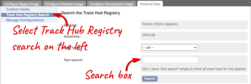
You can only find track hubs for the selected species and assembly denoted in the search box.

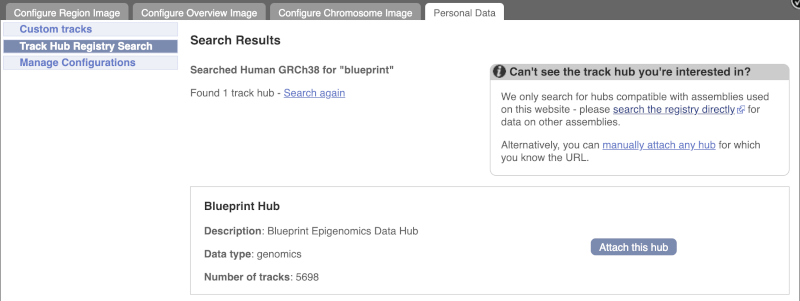
Search for blueprint.

Click Attach this hub in the search results page.

Track Hubs often contain vast amounts of data, which can slow Ensembl down, so only add them if you need them, and trash them when you are finished with them.

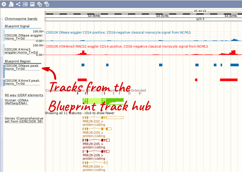
Go to Configure this Page to see that a new category has been added to your menu.

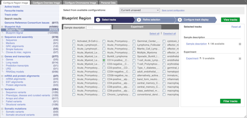
You can add tracks to the Region in Detail view using the matrix.

1. Add the ENCODE Track Hub to the ‘Region in Detail’ view for the genomic region surrounding the BRCA2 gene. Hint: You will need to add and view this Track Hub to the human GRCh37 genome assembly.

2. Turn on all the available tracks relating to Histone Modification Peaks and Transcription Factor Peaks in HeLa-S3 cells.

3. Which Transcription Factors and Histone Modifications have features in this region?

4. Add the Tracks showing Signals for the Histone Modifications and Transcription Factors that have peaks in this region. Compare the signal intensity to the location of annotated peaks.

5. Remove the ENCODE Track Hub from your list of custom tracks.

Upload the GD_wiggle.wig file to the Gluconacetobacter diazotrophicus PA1 5 (GCA_000021325) genome in Ensembl Bacteria. View this track across the region Chromosome:2884000-2898000. What is the highest score in this region?

Attach the file Spom_all_61G9EAAXX_and_61G9UAAXX.+.sorted.bam, which can be found here, to view in Schizoaccharomyces pombe. Go to the region I:490843-490870, can you see a mismatch between a read and the reference assembly?