Filter Events by Year
An introduction to the new Ensembl Genome Browser and custom annotation of variants with the Ensembl Variant Effect Predictor (VEP)
Course Details
- Lead Trainer
- Jorge Batista da Rocha
- Event Dates
- 2025-09-08 until 2025-09-10
- Location
- [BC]2 Basel Computational Biology Conference 2025
- Description
- Work with the Ensembl Outreach team to get hands-on experience accessing and analysing variation data with the new Ensembl genome browser and the Variant Effect Predictor (VEP).
- Survey
- An introduction to the new Ensembl Genome Browser and custom annotation of variants with the Ensembl Variant Effect Predictor (VEP) Feedback Survey
Demos and exercises
Exploring gene builds in Ensembl Beta
Exploring the MYH9 gene in Human
- In Ensembl Beta, find the MYH9 gene in the human GRCh38 (hg38) genome assembly.
- On which chromosome and which strand of the genome is this gene located?
- How many transcripts (splice variants) are there and how many of these are protein-coding?
- What’s the definition of MANE Select? How many coding exons does the MYH9 MANE Select transcript have?
- What sequences are available to download?
- Let’s explore the protein information that is available for the MANE Select transcript. Open the Entity Viewer.
- How long is the protein sequence (in aa) and what is the Ensembl protein ID?
- Open the Protein information panel under the ‘Gene function’ tab. What protein domain annotations are available for this transcript?
- What is the protein function according to UniProtKB?
- We’re going to explore homologues of the MYH9 gene. Open the ‘Gene relationships’ tab.
- Which species has the most similar sequence in terms of protein similarity? What is the corresponding gene ID?
- How many transcripts does the homologue have?
- Open the Species selector and enter
humanin the search box or click on the Human icon in the species list at the bottom of the page. Select to add the reference (GRCh38.p14) assembly and click on the green Add button. You should now see your selected species at the top of the page. Click on Find gene next to the species name, enter MYH9 in the search bar and click Go. In the results, click on MYH9 ENSG00000100345.23 and select Genome Browser. Click on the gene in the genome browser or click on the three dots (…) next to MYH9 protein_coding in the track panel on the right.- The gene is located on chromosome 22 on the reverse strand.
In the track panel, click on +22 transcripts to expand the list of transcripts.
- MYH9 has 23 transcripts. 6 of these are protein_coding (this includes the MANE select transcript) and 3 are defined as protein_coding_CDS_not_defined (a transcript that belongs to a protein_coding gene and does not contain an open reading frame).
In the track panel, click on the three dots (…) next to the MANE Select transcript to open the transcript panel and find out more details.
- The MANE Select is a default transcript per human gene that is representative of biology, well-supported, expressed and highly-conserved. The MANE Select transcript has 40 coding exons.
In the transcript panel, expand the Download option.
- You can download the genomic sequence and exons of the gene, and genomic sequence, cDNA (the sequence of the spliced exons of a transcript expressed in DNA notation – T rather than U – representing the coding or sense strand), exons, protein sequence and coding sequence (CDS) of the tanscript.
- To open the Entity Viewer, scroll to the bottom of the page and click on the Entity Viewer icon. Alternatively, if you are in the genome browser view, click on the first MYH9 transcript and click on View in Entity Viewer in the pop-up menu. Once in the Entity Viewer, click on the MANE Select transcript (this will open a grey information panel underneath).
- The protein is 1,960 aa long. The Ensembl protein ID is ENSP00000216181.6.
In the Entity Viewer, switch to the Gene function tab panel, click on the three dots (…) next to the MANE Select transcript to open the transcript panel and find out more details.
- Protein domains are distinct functional and/or structural units in a protein, which are usually responsible for a particular function or interaction, contributing to the overall role of a protein. There are several methods and algorithms that can be used to classify protein domains into families and functional sites. For the ENSP00000216181.6 protein, PANTHER and Pfam annotations are available.
In the Gene function tab, click on the UniProtKB/Swiss-Prot P35579 link to open the corresponding entry in UniProt.
- According to UniProtKB, the function of the protein is as follows: _Cellular myosin that appears to play a role in cytokinesis, cell shape, and specialized functions such as secretion and capping. Required for cortical actin clearance prior to oocyte exocytosis; promotes cell motility in conjunction with S100A4; and during cell spreading, plays an important role in cytoskeleton reorganization, focal contact formation (in the margins but not the central part of spreading cells), and lamellipodial retraction; this function is mechanically antagonized by MYH10.
- In the Entity Viewer, switch to the Gene relationships tab to view any homologues of the MYH9 gene. You can filter the homology table by header. The % protein similarity is the precentage of identical amino acid residues aligned against each other. Click on the % Protein similarity header once to sort the table in descending order.
- The Pan troglodytes (Chimpanzee) homologue is the most similar in terms of protein similarity. The gene ID of the homologue is ENSPTRG00000014309.6.
Click on the gene ID ENSPTRG00000014309.6, to open the corresponding homologue in the Entity Viewer. Count the number of transcripts you can see under the Transcripts tab.
- The chimp homologue has 4 transcripts.
Visualising a genomic region in human
Go to Ensembl Beta.
- Navigate to the region from 176,092,720 to 176,190,907 on the human GRCh38 assembly on chromosome 2. This region contains the HOXD gene cluster.
- How many HOXD genes can you find in this region?
- On a new browser tab, search for the gene cluster in GeneCards. What diseases are associated with the gene cluster? (Hint: you can search for gene clusters by adding an ‘@’ sign to the gene name, i.e.
HOXD@).
- Navigate to the HOXD1 gene. Let’s explore any overlapping regulatory features.
- Does this gene overlap any regulatory features? What type of regulatory element is this/are they?
- Downstream of the regulatory feature, should see a neighbouring regulatory element in the colour purple. What is this regulatory feature? How does it differ from an enhancer or promoter?
- Let’s explore variants found within the HOXD1 gene.
- What groups of variants can you find in the HOXD1 region?
- Zoom in on the first yellow-coloured variant. What type of variant is this and what are the alleles?
- What is the source of the variant? Can you provide the variant location in Variant Call Format (VCF)?
- In the Genome Browser app, click on the Navigate browser image icon in the track panel on the right. Expand Go to new location, select Chr 2, enter
176,092,720in Start and176,190,907in End. Click on the green Go button. Count the number of HOXD genes in the genome browser on the left.There are 9 HOXD genes on the forward and 1 HOXD gene on the reverse strand in this region.
Go to the GeneCards entry for the HOXD cluster. You can find diseases associate with the cluster in the Summaries for HOXD@ Gene section.
- The HOXD gene cluster is associated with synpolydactyly and clubfoot.
- In the genome browser, click on the HOXD1 (ENSG00000128645.15) gene and select Genome Browser in the pop-up menu. Scroll down to find the Regulatory track, which is indicated with the letter R on the far left. Click on the regulatory feature to see what type it is. Alternatively, you can find a legend in the track panel under the Regulation tab on the right.
The gene overlaps 1 regulatory feature: the promoter ENSR00000629037.
In the Regulation (R) track in the genome browser, click on the purple regulatory feature. The pop-up menu will tell you what type of regulatory feature this is. To find a description of the feature, go to the Regulation tab in the track panel on the right. Click on the three dots (…) next to TF binding.
- This regulatory feature is a TF binding site. These are sites that are enriched for Transcription Factor (TF) binding, but they lack epigenomic evidence to be classified as an enhancer or promoter
- In the genome browser, scroll down to the Variation (V) track. In the track, you should see green, yellow and salmon coloured variants. You can find a colour legend in the Variation tab in the track panel on the right.
The HOXD1 region overlaps various transcript, splicing and protein altering variants.
Using your mouse, zoom in on the first yellow-coloured variant. Click on the first yellow variant to find out more information about it.
- This variant (rs1691721387) is a single nucleotide variant (SNV). The reference allele is C and the alternative allele is T.
In the pop-up menu, select View in Entity Viewer to find out more information about the particular variant. In the track panel on the right, you can find the source of the variant (at the top) and the variant location in VCF (at the bottom).
- This rs1691721387 variant was imported from dbSNP (release 156). The VCF is as follows:
2 176188810 rs1691721387 C T.
Exploring genes in Bread wheat and its cultivars
- In Ensembl Beta, search for the
TraesCS2D02G248400gene in the Triticum aestivum (Bread wheat) IWGSC assembly.- How many transcripts are there?
- What is the definition of ‘Ensmebl canonical’? What does this gene do in Bread wheat?
- Align the protein sequence of the Ensembl canonical transcript to cultivars Cadenza, Julius and Paragon.
- How many hits are found in each of the cultivars?
- Download your BLAST results. What information can you find in the files?
- In the BLAST alignment file, what sequence does
Queryrefer to? What sequence doesSbjctrefer to?
- Open the Species selector and enter
bread wheatin the search box or click on the Bread wheat icon in the species list at the bottom of the page. Select to add the IWGSC assembly and click on the green Add button. You should now see your selected species at the top of the page. Click on Find gene next to the species name, enterTraesCS2D02G248400in the search bar and click Go. In the results, click on TraesCS2D02G248400 and select View in Genome Browser. You can find the number of transcripts in the genome browser view on the left, or the track panel on the right.TraesCS2D02G248400 has 2 transcripts.
Click on the three dots (…) next to the first transcript (TraesCS2D02G248400.2) in the track panel on the right. You can click on the questionmark (?) next to Ensembl canonical to find a description.
- The Ensembl canonical transcript is a single, representative transcript identified at every locus. The gene codes for an oxygen evolving enhancer protein.
- Stay in the transcript panel. Expand the Sequences option, select Protein sequence on the right and click on Blast whole sequence. This will take you to the BLAST app. Click on the blue Select species button and select the cultivars Cadenza, Julius and Paragon in Add species. In the BLAST app, click on the green Run button. Click on the blue Results button in the upper right-hand corner to view your results.
Cadenza has 3, Julius 10 and Paragon 3 hits.
Click on the Download icon next to the blue Results button in the upper right-hand corner. This will download your results in a compressed folder. Uncompress the folder and open the files using a plain text editor.
The folder containst 2 files: the
output.txtfile contains the BLAST alignments, including details about the sequence, alignment scores and statistics, and the sequence alignment. Thetable.tsvfile contains the metadata of your BLAST query, including any BLAST parameters and the results table you saw on the browser.Open the
output.txtfile.The Query (top sequence) refers to our sequence of interest (i.e. the protein in the IWGSC genome). The Sbjct (bottom sequence) refers to the homologue (the protein in the cultivar genome).
Exploring the Escherichia coli K-12 genome
Start in Ensembl Beta and select the Escherichia coli K-12 (ASM584v2) genome in the Species selector.
- Open the species information page.
- What substrain is this genome?
- What is the assembly (GCA_) ID? In what year was the the original K-12 isolate obtained?
- Find the era gene in E. coli K-12.
- Is the gene known under a different name?
- What are the coordinates for this gene?
- What is the biological function of the gene according to PDBe-KB?
- Go to Species selector and search for Escherichia coli by entering the species name in the search bar or by clicking on the species icon in the species list underneath. Select to add the species and click on the green Add button. You should now see the E. coli in your species list at the top of the page. Click on the blue Escherichia coli K-12 ASM584v2 to open the assembly information page. Open the track panel on the right.
The genome assembly is substrain MG1655.
Stay in the track panel. You can find the assembly ID under Assembly. Click on the assembly ID to open the corresponding entry in the European Nucleotide Archive (ENA), where the original sequence was submitted to.
The assembly ID is GCA_000005845.2. In the description in the ENA entry, we can see that MG1655 was derived from strain W1485, which was derived by Joshua Lederberg from the original K-12 isolate obtained from a patient in 1922.
- In the track panel, click on the Search icon, enter era into the text box and click on era b2566 in the results underneath.
The era_ gene in the E. coli K-12 genome is also known ‘b2566’ and the coordinates are 2,702,481-2,703,386.
In the pop-up menu, click on View in Entity Viewer. Switch to the Gene function tab and click on PDBe-KB P06616 to open the corresponding entry in PDBe-KB.
Accroding to PDBe-KB, the biological function is as follows: An essential GTPase that binds both GDP and GTP, with nucleotide exchange occurring on the order of seconds whereas hydrolysis occurs on the order of minutes. Plays a role in numerous processes, including cell cycle regulation, energy metabolism, as a chaperone for 16S rRNA processing and 30S ribosomal subunit biogenesis. This description is imported from UniProt.
Overview of Ensembl Beta
VEP
We have identified five variants on human chromosome nine, C-> A at 128203516, an A deletion at 128328461, C->A at 128322349, C->G at 128323079 and G->A at 128322917.
We will use the Ensembl VEP to determine:
- Have my variants already been annotated in Ensembl?
- What genes are affected by my variants?
- Do any of my variants affect gene regulation?
Go to the front page of Ensembl and click on the Variant Effect Predictor.
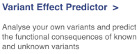
This page contains information about the VEP, including links to download the script version of the tool. Click on Launch VEP to open the input form:
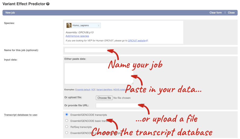
The data is in VCF format:
chromosome coordinate id reference alternative
Put the following into the Paste data box:
9 128328460 var1 TA T
9 128322349 var2 C A
9 128323079 var3 C G
9 128322917 var4 G A
9 128203516 var5 C A
The VEP will automatically detect that the data is in VCF.
There are further options that you can choose for your output. These are categorised as Identifiers, Variants and frequency data, Additional annotations, Predictions, Filtering options and Advanced options. Let’s open all the menus and take a look.
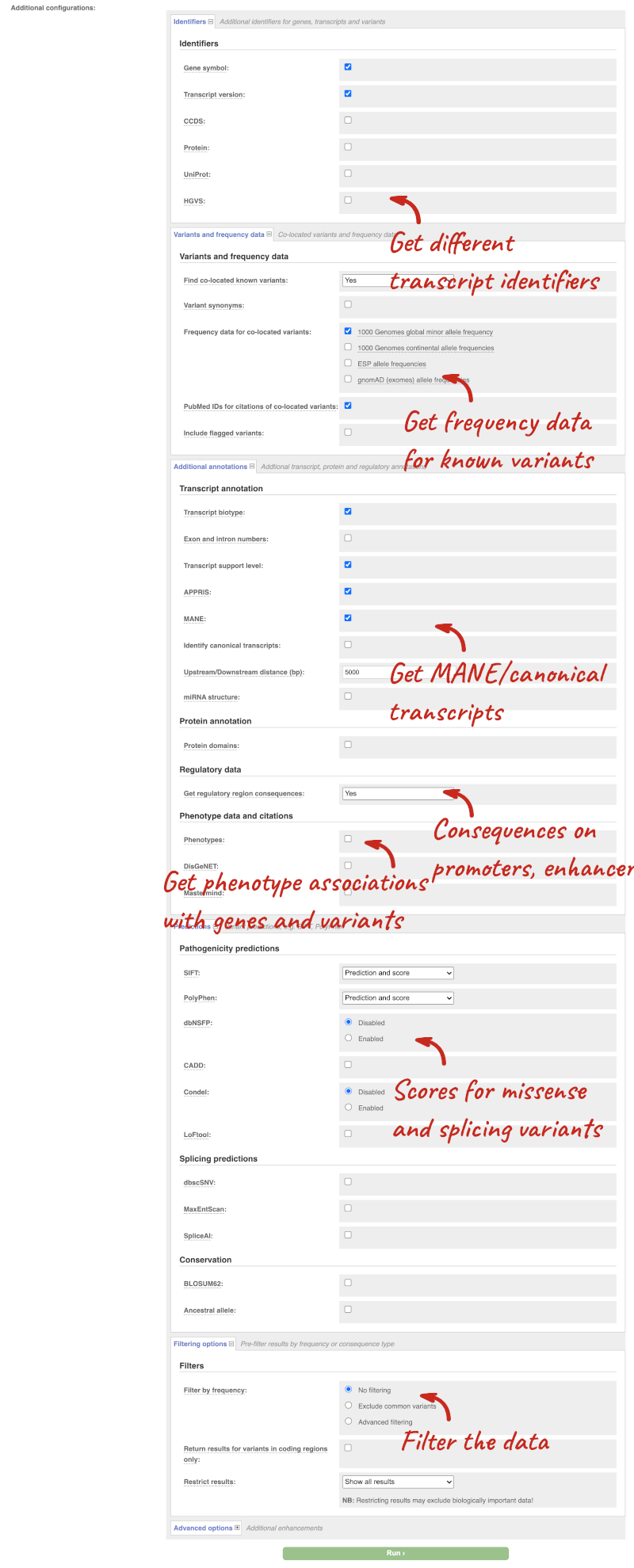
Hover over the options to see definitions.
We’re going to select some options:
- HGVS, annotation of variants in terms of the transcripts and proteins they affect, commonly-used by the clinical community
- Phenotypes
- Protein domains
When you’ve selected everything you need, scroll right to the bottom and click Run.
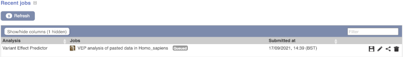
The display will show you the status of your job. It will say Queued, then automatically switch to Done when the job is done, you do not need to refresh the page. You can edit or discard your job at this time. If you have submitted multiple jobs, they will all appear here.
Click View results once your job is done.
In your results you will see a graphical summary of your data, as well as a table of your results.
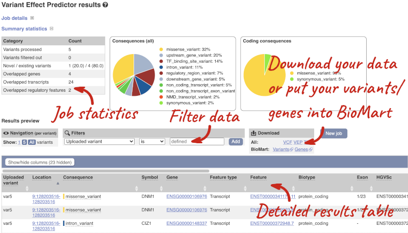
The results table is enormous and detailed, so we’re going to go through the it by section. The first column is Uploaded variant. If your input data contains IDs, like ours does, the ID is listed here. If your input data is only loci, this column will contain the locus and alleles of the variant. You’ll notice that the variants are not neccessarily in the order they were in in your input. You’ll also see that there are multiple lines in the table for each variant, with each line representing one transcript or other feature the variant affects.
You can mouse over any column name to get a definition of what is shown.
The next few columns give the information about the feature the variant affects, including the consequence. Where the feature is a transcript, you will see the gene symbol and stable ID and the transcript stable ID and biotype. Where the feature is a regulatory feature, you will get the stable ID and type. For a transcription factor binding motif (labelled as a MotifFeature) you will see just the ID. Most of the IDs are links to take you to the gene, transcript or regulatory feature homepage.
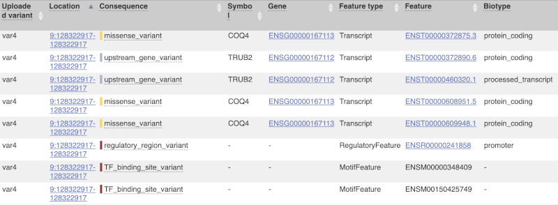
This is followed by details on the effects on transcripts, including the position of the variant in terms of the exon number, cDNA, CDS and protein, the amino acid and codon change, transcript flags, such as MANE, on the transcript, which can be used to choose a single transcript for variant reporting, and predicted pathogenicity scores. The predicted pathogenicity scores are shown as numbers with coloured highlights to indicate the prediction, and you can mouse-over the scores to get the prediction in words. Two options that we selected in the input form are the HGVS notation, which is shown to the left of the image below and can be used for reporting, and the Domains to the right. The Domains list the proteins domains found, and where there is available, provide a link to the 3D protein model which will launch a LiteMol viewer, highlighting the variant position.
![]()
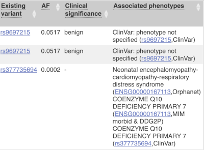
Where the variant is known, the ID of the existing variant is listed, with a link out to the variant homepage. In this example, only rsIDs from dbSNP are shown, but sometimes you will see IDs from other sources such as COSMIC. The VEP also looks up the variant from frequency files, and pulls back the allele frequency (AF in the table), which will give you the 1000 Genomes Global Allele Frequency. In our query, we have not selected allele frequencies from the continental 1000 Genomes populations or from gnomAD, but these could also be shown here. We can also see ClinVar clinical significance and the phenotypes associated with known variants or with the genes affected by the variants, with the variant ID listed for variant associations and the gene ID listed for gene associations, along with the source of the association.
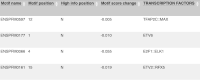
For variants that affect transcription factor binding motifs, there are columns that show the effect on motifs (you may need to click on Show/hide columns at the top left of the table to display these). Here you can see the position of the variant in the motif, if the change increases or decreases the binding affinity of the motif and the transcription factors that bind the motif.
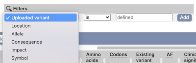
Above the table is the Filter option, which allows you to filter by any column in the table. You can select a column from the drop-down, then a logic option from the next drop-down, then type in your filter to the following box. We’ll try a filter of Consequence, followed by is then missense_variant, which will give us only variants that change the amino acid sequence of the protein. You’ll notice that as you type missense_variant, the VEP will make suggestions for an autocomplete.
You can export your VEP results in various formats, including VCF. When you export as VCF, you’ll get all the VEP annotation listed under CSQ in the INFO column. After filtering your data, you’ll see that you have the option to export only the filtered data. You can also drop all the genes you’ve found into the Gene BioMart, or all the known variants into the Variation BioMart to export further information about them.
Running CFTR variants through VEP
Resequencing of the genomic region of the human CFTR (cystic fibrosis transmembrane conductance regulator (ATP-binding cassette sub-family C, member 7) gene (ENSG00000001626) has revealed the following variants. The alleles defined in the forward strand:
- G/A at 7: 117,530,985
- T/C at 7: 117,531,038
- T/C at 7: 117,531,068
Use the VEP tool in Ensembl and choose the options to see SIFT and PolyPhen predictions. Do these variants result in a change in the proteins encoded by any of the Ensembl genes? Which gene? Have the variants already been found?
Go to the Ensembl homepage and click on the link Tools at the top of the page. Currently there are nine tools listed in that page. Click on Variant Effect Predictor and enter the three variants as below:
7	117530985	117530985	G/A
7	117531038	117531038	T/C
7	117531068	117531068	T/C
Note: Variation data input can be done in a variety of formats. See more details about the different data formats and their structure in this VEP documentation page. Click Run. When your job is listed as Done, click View Results.
You will get a table with the consequence terms from the Sequence Ontology project (http://www.sequenceontology.org/) (i.e. synonymous, missense, downstream, intronic, 5’ UTR, 3’ UTR, etc) provided by VEP for the listed SNPs. You can also upload the VEP results as a track and view them on Location pages in Ensembl. SIFT and PolyPhen are available for missense SNPs only. For two of the entered positions, the variations have been predicted to have missense consequences of various pathogenicity (coordinate 117531038 and 117531068), both affecting CFTR. All the three variants have been already annotated and are known as rs1800077, rs1800078 and rs35516286 in dbSNP (databases, literature, etc).
VEP analysis of structural variants in human
We have details of a genomic deletion in a breast cancer sample in VCF format:
13 32307062 sv1 . <DEL> . . SVTYPE=DEL;END=32908738
Use VEP in Ensembl to find out the following information:
1. How many genes have been affected?
2. Does the structural variant (SV) cause deletion of any complete transcripts?
3. Map your variant in the Ensembl browser on the Region in detail view.
- Click on VEP at the top of any Ensembl page and open the web interface. Make sure your species is Human. It is good practise to name your VEP jobs something descriptive, such as Patient deletion exercise. Paste the variant in VCF format into the Paste data field and hit Run.
12 different genes are affected by the SV.
- Filter your table by select Consequence is
transcript_ablationat the top of the table and click Add.Yes, there is deletion of complete transcripts of PDS5B, N4BP2L1, BRCA2, RNY1P4, IFIT1P1, ATP8A2P2, N4BP2L2, N4BP2L2-IT2 and one gene without official symbols: ENSG00000212293.
- To view your variant in the browser click on the location link in the results table 13: 32307062-32908738. The link will open the Region in detail view in a new tab. If you have given your data a name it will appear automatically in red. If not, you may need to Configure this page and add it under the Personal data tab in the pop-up menu.
VEP CMD Human
Command-line VEP analysis of variants from a 1000 Genomes Project dataset
Ensembl’s Variant Effect Pedirctor (VEP) is a powerful tool for annotating genomic variants. VEP is accessible via web, REST API and command line options.
In this practical session, we will practice using VEP via command line to annotate a variant call file (VCF).
The VCF you will use contains variant calls for Homo Sapiens chromosome 13 from the IGSR: The International Genome Sample Resource. This file was extracted using Ensembl’s Data Slicer for human variation aligned to GRCh38, with the IGSR British in England and Scotland GBR population samples subsetted. The file is available here
Installation of Docker and VEP:
For this tutorial, we will be using VEP as installed by Docker.
To run the analysis on your computer, you will need to have installed Docker. Docker requires you to have admistration controls of the computer you install it on. It is available as a command line tool and via desktop interfaces, please see the Docker guides for more info. You may use Docker for Windows and the Windows subsystem for Linux, Docker for Mac, or Docker for Linux. Please install whichever version suits your system.
Once docker is installed, you will need to install VEP via using Dockerusing the linked instructions.
If you get stuck at these steps, ask your trainer for help, or share a computer with another participant who has it working.
Directories and files required:
You must create a volume space for VEP to access as a linked volume to the docker:
mkdir $HOME/vep_data
Once you have created this directory, you can run the following command to start an interactive job where we will run the following commands in this tutorial.
docker run -t -i -v $HOME/vep_data:/data ensemblorg/ensembl-vep
Note - In the example above, data in $HOME/vep_data will be accessible by both the local machine and VEP Docker. The Ensembl VEP API, plugins and their dependencies (e.g. Perl APIs, Bio::DB::HTS, htslib, …) are already installed in the image.
The subsetted IGSR VCF file name is: 13.32315086-32400268.ALL.chr13_GRCh38.genotypes.20170504.GBR.vcf
You can download it into the docker volume with
curl https://ftp.ebi.ac.uk/pub/databases/ensembl/training/output_files/13.32315086-32400268.ALL.chr13_GRCh38.genotypes.20170504.GBR.vcf
Tutorials for using VEP:
A General Tutorial for command line VEP is available to try out or compare to if you needsome guidance.
You can use the options guide at Ensembl VEP Options to help find the commands you need.
Note - the commands below do not make use of VEP caches, this is for the sake of easier install for this tutorial, but in practical applications, VEP caches will greatly improve run speed.
Exercises:
- Explore the VCF file with any text viewer to explore its contents. What do lines denoted by “##” represent? What are the key headers in the file?
You can use VCF file specifications as a reminder.
- Use the command-line VEP tool to annotate the variants in the IGSR VCF file. Here is an example command:
vep -i [input_file] -o [output_file] --database --symbol
We recommend using the default VEP output format, as it’s easier to read on screen, but you can preserve the output as VCF by using --vcf.
-
Explore the output of VEP in any text viewer to explore the contents. What genes are affected by the variants in the file? Why are there multiple results for each variant?
-
Re-run the command-line VEP tool to annotate the variants in your VCF including if they occur in a MANE and Ensembl Canonical transcript. Save the output of this query into a separate output file in the default text format (omit –vcf).
-
Use the
filter_VEPtool to find variants that are located within the BRCA2 gene in a MANE transcript. Are there any missense variants present in this filter?
- From the original output of exercise 2, what has been the overall effect of adding annotations and then filtering using that information?
- Are there any missense variants left?
Bonus!
If you finish all that, try pasting the variant below into Web VEP and select the alphamissense, revel, CADD, mavedb and mutfunc options.
What do you see in the results?
13 48040982 . A T
Exercise 1
You can open the VCF file with any text editor, or by using a command such as: vim 13.32315086-32400268.ALL.chr13_GRCh38.genotypes.20170504.GBR.vcf. Then use the arrow keys to navigate. When done, use the ESC key to switch to normal mode, then write :q! (quit without saving). Lines starting with ## indicate information headers, which contain information about the file content and how it was processed.
Exercise 2
vep -i 13.32315086-32400268.ALL.chr13_GRCh38.genotypes.20170504.GBR.vcf -o VEP_annot_chr13_GBR.vcf --database
Your own script may not look exactly like this and you may employ different flags, here are some common examples:
--input_fileor-iAllows you to specify the location of the input file.--output_fileor-oAllows you to specify the name of the output file.--force_overwriteAllows VEP to overwrite a pre-existing output file with the same name.--genomesPoints VEP to the Ensembl Genomes (non-vertebrates) server. (not used for this homo sapiens example)--databaseEnable VEP to use local or remote databases.--cacheEnables the use of the cache (this can speed up VEP significantly - not used here for install simplicity).--cache_versonAllows you to specify the cache version. This should be used with Ensembl Genomes caches, since their version numbers do not match Ensembl versions. For example, the VEP/Ensembl version may be 110 and the Ensembl Genomes version 57.--check_existingChecks for the existence of known variants that are co-located with your input variants.--offlineEnables offline mode (no database connections are made).
Exercise 3
You may use a similar less command or method to open the annotated VCF file:
less -S VEP_annot_chr13_GBR.vcf
There are two genes listed in the annotations, ZAR1L ENSG00000189167 and BRCA2 ENSG00000139618. There are multiple rows for each variant representing the variant consequence in different transcripts.
Exercise 4
Rerun VEP with the following command:
vep -i 13.32315086-32400268.ALL.chr13_GRCh38.genotypes.20170504.GBR.vcf -o VEP_annot_chr13_GBR_MANE_Can.txt --canonical --mane --symbol --database
Exercise 5
Filter for BRCA2 and MANE with the following command:
filter_vep -i VEP_annot_chr13_GBR_MANE_Can_gnomadAF.txt -o VEP_annot_FILT.txt --filter "((SYMBOL is BRCA2) and (MANE_SELECT exists))"
By adding transcript set and gene symbol then using filters based on these, we can reduce the annotated variant set down.
To filter to include only the missense results you could add and (Consequence is missense_variant) to the command above.
There is a missense variant - rs80358762 - you can explore phenotype information related to that variant here. Note that although it’s a rare missense variant in BRCA2, the evidence from multiple ClinVar submitters indicate that it is benign.
Bonus!
This variant is novel and does not have an accessioned ID and is not present in the allele frequency resources. Consider just the missense variant in NUDT15, you can see that prediction tools we enabled(alphamissense, revel and CADD) are all relatively low scores, below those that would normally be thought of as pathogenic. However, some ofthe IntAct and MaveDB scores - which are based on experimental data - indicate that the protein structure is significantly impacted, suggesting this variant may merit further investigation.
VEP CMD Beta CHM13T2T
Command-line VEP analysis of variants against the CHM13 Telomere to Telomere Genome
Please note - it is best to attempt this practical AFTER attempting the practical “VEP CMD Human” for 1000 Genomes Variants on the GRCh38 human reference genome.
Ensembl’s Variant Effect Pedirctor (VEP) is a powerful tool for annotating genomic variants. VEP is accessible via web, REST API and command line options.
In this practical session, we will practice using VEP via command line to annotate a variant call file (VCF) containing a short list of variants which were mapped to the CHM13 Telomere to Telomere Genome. This example file is available here
For more info, there is a blog about running Ensembl VEP for alternative human assemblies and a guide for running VEP on the HPRC assemblies.
Installation of Docker and VEP:
For this tutorial, we will be using VEP as installed by Docker.
To run the analysis on your computer, you will need to have installed Docker. Docker requires you to have admistration controls of the computer you install it on. It is available as a command line tool and via desktop interfaces, please see the Docker guides for more info. You may use Docker for Windows and the Windows subsystem for Linux, Docker for Mac, or Docker for Linux. Please install whichever version suits your system.
Once docker is installed, you will need to install VEP via using Dockerusing the linked instructions.
If you get stuck at these steps, ask your trainer for help, or share a computer with another participant who has it working.
Directories and files required:
You must create a volume space for VEP to access as a linked volume to the docker:
mkdir $HOME/vep_data
Once you have created this directory, you can run the following command to start an interactive job where we will run the following commands in this tutorial.
docker run -t -i -v $HOME/vep_data:/data ensemblorg/ensembl-vep
Note - In the example above, data in $HOME/vep_data will be accessible by both the local machine and VEP Docker. The Ensembl VEP API, plugins and their dependencies (e.g. Perl APIs, Bio::DB::HTS, htslib, …) are already installed in the image.
You will require the following files from Ensembl FTP directory for VEP for the CHM13 Assembly
The GFF file (contains gene annotations) and its index:
curl -O https://ftp.ebi.ac.uk/pub/ensemblorganisms/Homo_sapiens/GCA_009914755.4/vep/ensembl/geneset/2022_07/genes.gff3.bgz
curl -O https://ftp.ebi.ac.uk/pub/ensemblorganisms/Homo_sapiens/GCA_009914755.4/vep/ensembl/geneset/2022_07/genes.gff3.bgz.csi
The fasta sequence file (bgzipped) for CHM13 and its index :
curl -O https://ftp.ebi.ac.uk/pub/ensemblorganisms/Homo_sapiens/GCA_009914755.4/vep/genome/softmasked.fa.bgz
curl -O https://ftp.ebi.ac.uk/pub/ensemblorganisms/Homo_sapiens/GCA_009914755.4/vep/genome/softmasked.fa.bgz.gzi
There is a VEP cache avaiable for CHM13 available to add more VEP annotation info:
curl -O https://ftp.ensembl.org/pub/rapid-release/species/Homo_sapiens/GCA_009914755.4/ensembl/variation/2022_10/indexed_vep_cache/Homo_sapiens-GCA_009914755.4-2022_10.tar.gz
Place this into the vep_data folder and uncompress:
tar xzf Homo_sapiens-GCA_009914755.4-2022_10.tar.gz
If you havent as yet, get the example file into the practical: curl -O https://ftp.ebi.ac.uk/pub/databases/ensembl/training/output_files/example_vars_CHM13T2T.txt
Tutorials for using VEP:
A General Tutorial for command line VEP is available to try out or compare to if you needsome guidance.
You can use the options guide at Ensembl VEP Options to help find the commands you need.
Note - the commands below do not make use of VEP caches, this is for the sake of easier install for this tutorial, but in practical applications, VEP caches will greatly improve run speed.
Exercises:
-
Explore the example file, how many variants are listed in the file? Are any multi-allelic?
-
Use the command-line VEP tool to annotate the variants in the file and output format with the GFF and sequence fasta. Include the gene symbol. Here is an example command:
vep -i [input_file] -o [output_file] --gff [gene annotation file] --fasta [genomic sequence fasta file]
-
Explore the output of VEP in any text viewer to explore the contents. Are the identifiers of the genes the same as for what you found in GRCh38? What are the consequences of variants are present in the file?
-
Now include the use of the cache, and include the option to label canonical transcripts. You will need to include the options to direct to the cache
--species homo_sapiens_gca009914755v4 --cache_version 107 -
Now run a filter VEP command to filter for variants in BRCA and canonical transcripts. How many variants remain?
Exercise 1
You can open the example file with any text editor, or by using a command such as: less example_vars_CHM13T2T.txt. Then use the arrow keys to navigate. When done, use the ESC key to switch to normal mode, then write :q! (quit without saving). There are 5 variants in this example file. rs1230223847 lists two possible allele changes, A > C and A > T.
Exercise 2
vep -i example_vars_CHM13T2T.txt --gff genes.gff3.bgz --fasta softmasked.fa.bgz -o chm13_example_variants.txt --symbol
Your own script may not look exactly like this and you may employ different flags, here are some common examples:
--input_fileor-iAllows you to specify the location of the input file.--output_fileor-oAllows you to specify the name of the output file.--force_overwriteAllows VEP to overwrite a pre-existing output file with the same name.--genomesPoints VEP to the Ensembl Genomes (non-vertebrates) server. (not used for this homo sapiens example)--databaseEnable VEP to use local or remote databases.--cacheEnables the use of the cache (this can speed up VEP significantly).--cache_versonAllows you to specify the cache version. This should be used with Ensembl Genomes caches, since their version numbers do not match Ensembl versions. For example, the VEP/Ensembl version may be 110 and the Ensembl Genomes version 57.--check_existingChecks for the existence of known variants that are co-located with your input variants.--offlineEnables offline mode (no database connections are made).
Exercise 3
You may use a similar less command or method to open the annotated VCF file:
less -S chm13_example_variants.txt
There are two genes listed in the annotations, ZAR1L ENSG05220054524 and BRCA2 ENSG05220054575. These are different IDs to those in GRCh38. The consequences include: 5_prime_UTR_variant downstream_gene_variant frameshift_variant intron_variant missense_variant splice_acceptor_variant synonymous_variant upstream_gene_variant
Exercise 4
Rerun VEP with the following command:
vep -i example_vars_CHM13T2T.txt --offline --species homo_sapiens_gca009914755v4 --cache_version 107 --fasta chm13_softmasked.fa.bgz --symbol --canonical -o example_vars_CHM13T2T_cache_CAN.txt
Exercise 5
filter_vep -i example_vars_CHM13T2T_cache_CAN.txt --filter "(SYMBOL is BRCA2) and (CANONICAL = YES)" -o example_vars_CHM13T2T_FILT_CAN_BRCA.txt
There are six variants remaining in the file. The multi-allelic rs1230223847 is listed for each of its alleles. Congratulations - you can now annotate variants on the Telomere to Telomere human genome!