Filter Events by Year
Ensembl Browser Workshop - Livestock Pangenomics 2024
Course Details
- Lead Trainer
- Louisse Paola Mirabueno
- Associate Trainer
- Event Date
- 2024-07-25
- Location
- Piacenza, Italy
- Description
- Work with the Ensembl team to learn about pangenome gene annotation and explore how to access pangenome data in the Ensembl browser.
Demos and exercises
Species and genome assemblies
Demo: Introduction to Ensembl
Ensembl
Homepage
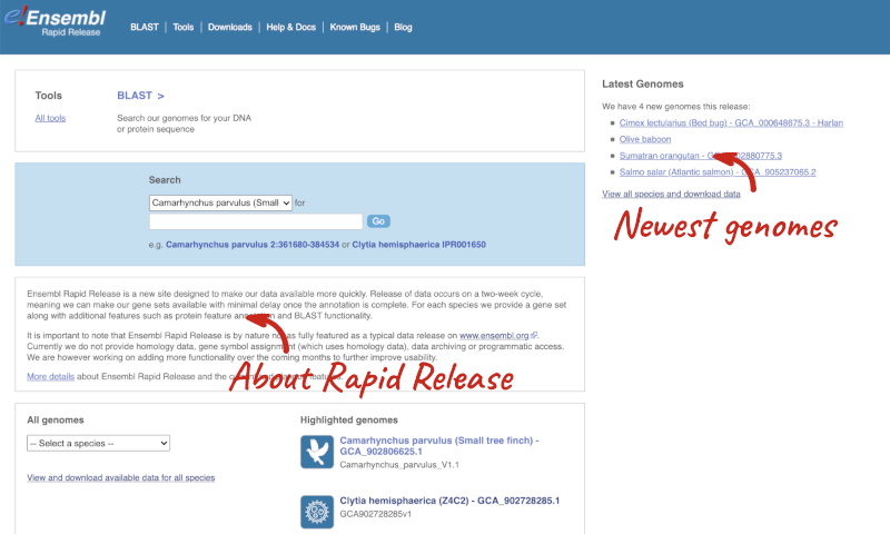
The homepage of Ensembl is found at www.ensembl.org. It contains lots of information and links to help you navigate Ensembl:
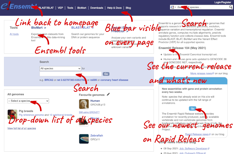
On the right-hand panel you can see the current release number and what has come out in this release. To access old releases, scroll to the bottom of the page and click on View in archive site in the right-hand corner.
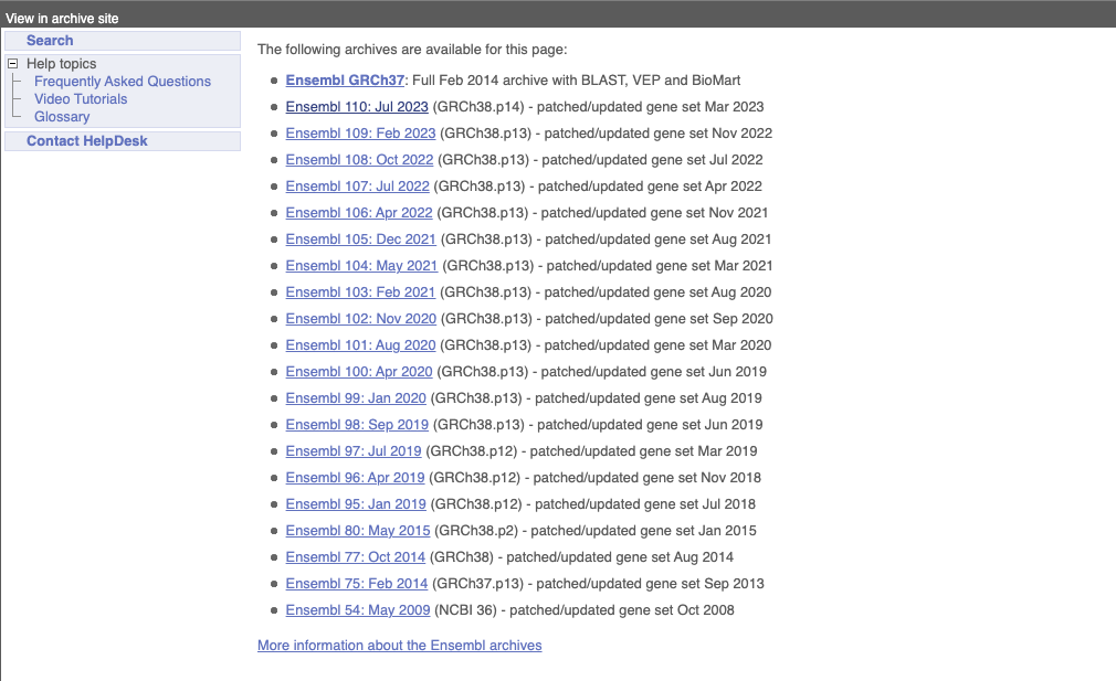
Click on the links to go to the archives. Alternatively, you can jump quickly to the correct release by adding e plus the release number in the URL. For example e98.ensembl.org jumps to Ensembl release 98.
Available pangenomes
Pangenomes are available for:
- Canis lupus familiaris (Dog): 4 additional breeds
- Gallus gallus (Chicken): 2 additional breeds
- Mus musculus (Mouse): 15 additional strains
- Ovis aries (Sheep): 1 additional breed
- Rattus norvegicus (Norway rat): 3 additional strains
- Sus scrofa (Pig): 12 additional breeds
To view all available species in Ensembl, scroll back up to the top of the homepage and click the View full list of all species link underneath the coloured search block.
You can search for your species of interest (either the common or scientific name) using the search bar at the top right-hand corner of the table. Click on the common name of your species of interest to go to the species information page. We’ll click on Pig.
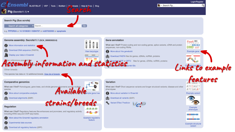
This is the species information page for Pig. Here you can see links to example features and to download flatfiles. Under the Genome assembly section, we can see that the species has data on an additional 12 breeds. Click on View list of breeds to see all available breeds in tabular form.
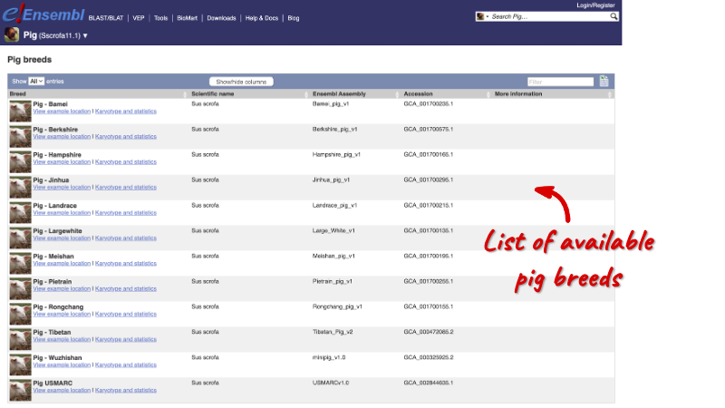
Species information
Let’s focus on the Genome assembly. Go back to the species information page and click on More information and statistics under the Genome assembly section.

Here you’ll find a detailed description of how to the genome was produced and links to the original source. You will also see details of how the genes were annotated.
Ensembl Plants
Homepage
Let’s take a look at the Ensembl Plants homepage at plants.ensembl.org.
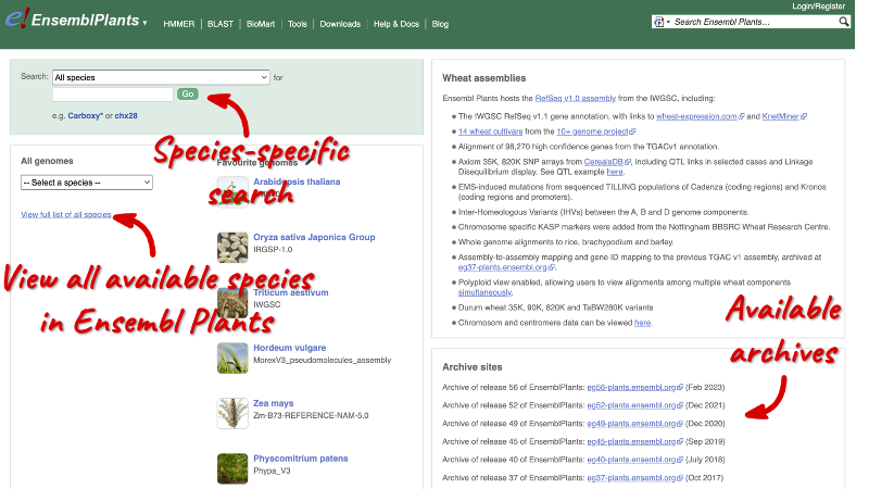
You will notice that the Ensembl Plants website is structured very similarly to the Ensembl main site. The only difference being the colour-coding.
You can navigate most of the taxa in the same way as you would with Ensembl.
Available pangenomes in Ensembl Plants
Pangenomes are available for:
- Hordeum vulgare (Barley): 2 additional cultivars
- Oryza sativa (Rice): 15 additional cultivars
- Triticum aestivum (Wheat): 17 additional cultivars
To view all available species, go to the Ensembl Plants homepage and click the View full list of all species link underneath the coloured search block.
Ensembl Rapid Release
Our newest genomes, such as those coming from the Darwin Tree of Life, are available on rapid.ensembl.org. Note that Ensembl Rapid Release has fewer features and tools available compared to Ensembl and Ensembl Genomes. Only gene annotation data is available, and variation and comparative genomics data is limited.
The Ensembl Projects page, lists all projects and collaborations that incorporate Ensembl gene annotation, including consortia with a focus on livestock and agriculture:
- AQUA-FAANG
- GENE-SWitCH
- BovReg
- NextGen
Available data, including genebuilds, from the Human Pangenome Reference Consortium (HPRC) can be accessed via projects.ensembl.org/hprc.
Pig species data
-
How many coding and non-coding genes does pig have?
-
When was the current Sus scrofa genome assembly produced and by whom?
1.Select Pig from the drop down species list, or click on View full list of all Ensembl species, then choose Pig from the list to go to the species homepage. Click on More information and statistics.
Pig has 22,063 coding genes and 13,154 non-coding genes.
- The Sscrofa11.1 assembly of the pig genome was produced in January 2017 by the Swine Genome Sequencing Consortium (SGSC).
Gallus gallus (Chicken) breeds
-
Which Gallus gallus (Chicken) breeds are available?
-
When was the genebuild of the Reg Jungle fowl last updated?
- On the Ensembl homepage, select Chicken from the drop-down species list, or click on View full list of all Ensembl species and click on Chicken from the table to go to the species information page. Under the Genome assembly section, click on View list of breeds.
Two additional Chicken breeds are available: White leghorn layer and Red Jungle fowl.
- On the Ensembl homepage, click on View full list of all Ensembl species. Search for Red Jungle fowl and open the species information page. Click on More information and statistics under the Genome assembly section. In the right-hand panel under Summary, look for **Genebuild last updated/patched.
The genebuild for Red Jungle fowl was last updated in January 2022.
Triticum aestivum (wheat) cultivars
-
Are there any additional cultivars available alongside the Triticum aestivum (IWGSC) reference genome?
-
Find the description of the wheat assembly. Which institute provided the assembly and annotations?
-
How many coding and non-coding genes does the IWGSC assembly have?
-
Are there any other species of the genus Triticum available in Ensembl? If so, which species are they?
- Go to Ensembl Plants and click on Triticum aestivum on the front page of Ensembl Plants to go to the species information page. Under the Genome assembly section of the species page, you will find the number of cultivars in wheat.
There are 14 cultivars.
- Click on More information and statistics in the Genome assembly section and scroll down to the paragraph on Assembly.
The assembly and annotations were generated by the International Wheat Genome Sequencing Consortium (IWGSC).
- Stay on the More information and statistics page. You can find some summary statistics on the right-hand side.
The T. aestivum (IWGSC) assembly has 107,891 coding and 12,853 non-coding genes.
- Go to the Ensembl Plants homepage. Click on View full list of all species in the All genomes panel. Filter the table by entering
Triticumin the text box on the top right-hand corner of the table.Besides T. aestivum are 4 other Triticum species available in Ensembl: Triticum dicoccoides (wild emmer wheat), Triticum spelta (spelt), Triticum turgidum (domesticated emmer wheat) and Triticum urartu (red wild einkorn wheat).
Oryza sativa (Rice) cultivars
-
How many Oryza sativa genomes are available in Ensembl Plants?
-
How many cultivars are available for the Oryza sativa Japonica group?
-
What is the GCA ID of Oryza sativa (Geng/Japonica-trop2 var. Ketan Nangka)?
- Go to Ensembl Plants and click on View full list of all species on homepage. Enter Oryza sativa in the filter in the top right-hand corner of the table.
17 O. sativa genomes are available in Ensembl Plants.
- Go back to the species list and search for Oryza sativa Japonica using the table’s filter. Click on Oryza sativa Japonica Group to open the species information page. Under the Genome assembly section, look for the number of cultivars.
15 additional cultivars are available.
- Click on View list of cultivars. Look for the Ketan Nangka cultivar.
The GCA ID is GCA_009831275.1.
Exploring genomic regions
Demo: Exploring a genomic region in Pig
Searching for a region
Start at the Ensembl homepage, www.ensembl.org. In the species-specific search box, select Pig from the drop-down menu, enter 15:81890000-82000000 into the search box and click on Go. The format of your coordinates should be:
chromosome:start-end
You do not need to remove commas if there are any.
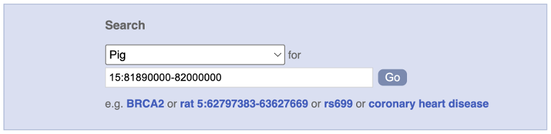
Press Enter or click Go to jump directly to the Region in detail page in Pig.
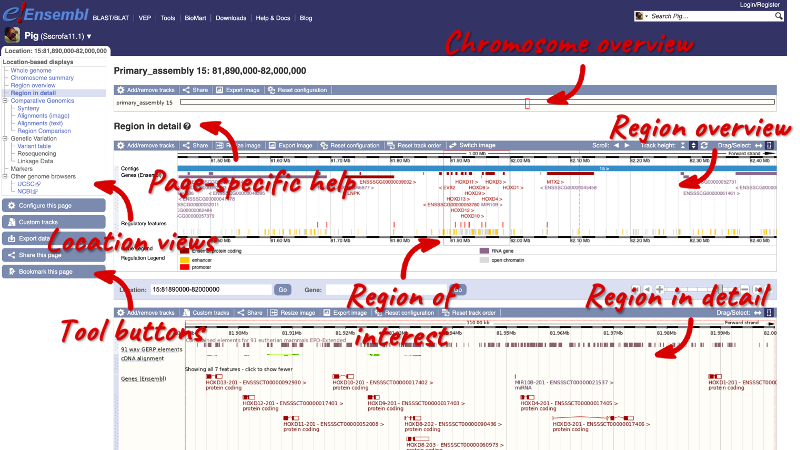
Region in detail
Click on the questionmark button  button to view page-specific help. The help pages provide descriptions, labelled images and, in some cases, help videos to exaplin what you can see on the page and how to interact with it.
The Region in detail page is made up of three images, let’s look at each one in detail.
Chromosome overview
The first image shows the chromosome overview:
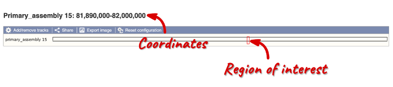
You can jump to or highlight a different region by dragging out a box in the image using your cursor. Click and drag a box on the chromosome. A pop-up menu will appear.
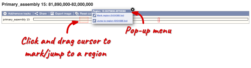
If you want to move to the region, you can click on Jump to region (### bp). If you want to highlight it, click on Mark region (###bp). For now, we’ll close the pop-up by clicking on the X on the corner.
Region overview
The second image shows a 1Mb region overview around our region of interest, which is marked in a red border. This view allows you to scroll back and forth along the chromosome.
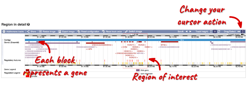
You can also drag out and jump to or mark a region.
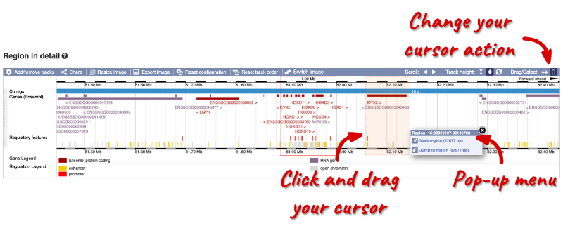
Click on the X to close the pop-up menu.
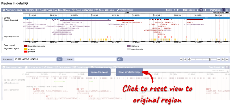
Click on the Drag/Select button  to change the action of your mouse click. Click on the arrows to scroll along the chromosome by clicking and dragging your cursor within the region overview image. As you do this you’ll see the image below grey out and two blue buttons appear. Clicking on Update this image would jump the lower image to the region you scrolled to. We want to go back to where we started, so we’ll click on Reset scrollable image.
Region in detail view
The third image is a detailed, configurable view of the region.
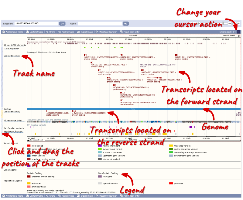
Click on the Drag/Select option at the top right-hand corner to switch mouse action. Similarly to the region overview, you can select Drag, to scroll along the genome (the page will reload when you drop the mouse button). On Select you can drag out a box to highlight or zoom in on a region of interest.
Set your cursor action to Select, drag out a box around an exon and select Mark region.
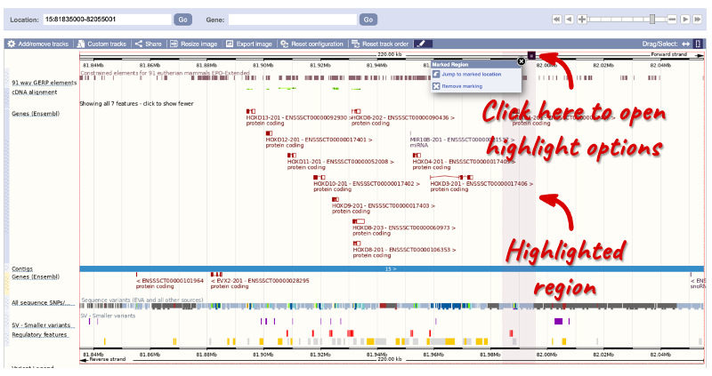
The highlight will remain in place if you zoom in and out or move around the region. This allows you to keep track of regions or features of interest.
Configuring the region view
We can edit what we see on this page by clicking on the blue Configure this page menu at the left.

This will open a menu that allows you to change the image.
You can put some tracks on in different styles; more details are in this FAQ: http://www.ensembl.org/Help/Faq?id=335.
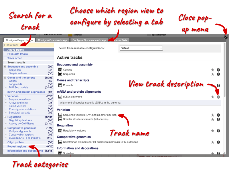
Let’s add some tracks to this image. Add the All variants on genotyping chips - short variants (SNPs and indels) track in the pop-up menu. You can use the search bar to filter for the track, or you can select the track in the left-hand menu under Variation > Arrays and other. To enable the track, click on the square next to the track name and select the track style Normal.
Now click on the check icon in the top right-hand corner to save and close the menu. Alternatively, click anywhere outside of the pop-up menu. Wait for the Region in detail view to load. Once loaded, you should be able to see the track in the image. If the track does not appear in the image, no track features are present in your region of interest. You may need to scroll along the genome or zoom out to visualise a broader region.
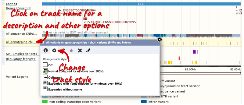
We can also change the way the tracks appear by hovering over the track name then the cog wheel to open a menu. We can move tracks around by clicking and dragging on the bar to the left of the track name.
Sharing and exporting
Now that you’ve got the region view how you want it, you might like to show something you’ve found to a colleague or collaborator. Click on the Share this page button (either in the left-hand panel or at the top of the Region in detail view) to generate a URL. You can share the URL with your colleague, so that they can see the same view as you (including all the tracks and configurations you’ve added). The URL contains the Ensembl release number, so if a new release or even assembly comes out, your link will just take you to the archive site for the release it was made on.

You can also export the region image by clicking on the Export image button at the top of the Region in detail view, or export the data (i.e. the sequence or the annotation) by clicking on the Export data button in the left-hand panel.
To return this to the default view, go to click on Reset configuration at the top of the Region in detail view.
Exploring a genomic region in Sus scrofa (Pig)
-
Go to the region from 8,805,953 to 8,858,418 on pig chromosome 11.
-
Configure this page to turn on the Tandem repeats (TRF) track in this view. What is this track? How many TRF overlap this region?
-
Create a URL for this display. Email it to your neighbour.
-
Export the genomic sequence of the region you are looking at in FASTA format.
-
Turn off all tracks you added to the Region in detail page.
-
Go to the Ensembl homepage. Select Pig from the drop-down menu in the blue box and enter
11:8,805,953-8,858,418in the text box. Click Go. - Click Configure this page in the left-hand menu (or on Add/remove tracks at the top left-hand corner of the Region in detail image). Type TRF into the search field in the top left-hand corner of the pop-up menu. Enable the Tandem repeats (TRF) track on the right. You can click on the i icon on the far left for a track description.
The TRF track locates adjacent copies of a pattern of nucleotides. Save and close the new configuration by clicking on the check icon in the top right-hand corner of the pop-up menu or by clicking anywhere outside the pop-up menu. There are 19 TRF that overlap this region.
-
Click Share this page in the left hand-side panel. Copy the URL, get your neighbour’s email address and send them the URL you copied. When you receive the link from them, open the email and click on your link. You should be able to view the page with the new configuration and data tracks they have added.
-
Click on Export data in the left-hand menu. Leave the default parameters as they are. Click Next> and view the sequence in a new browser tab by clicking on Text. The sequence is in FASTA formatwhich comprises a header (beginning with >) that provides information about the genome assembly (primary_assembly:Sscrofa11.1), the chromosome, the start and end coordinates and the strand. For example:
>primary_assembly:Sscrofa11.1:11:8805953-8858418:1 - Click on Reset configuration at the top of the Region in detail image.
Exploring a genomic region in Gallus gallus (Chicken)
-
Go to the region from 38,111,022-38,265,293 on chicken chromosome 5. How many contigs make up this portion of the assembly (contigs are contiguous stretches of DNA sequence that have been assembled solely based on direct sequencing information)?
-
Zoom in on ESRRB gene.
-
Turn on the RefSeq GFF3 annotation track as Expanded with labels.
-
Save this image in PDF format.
- Go to the Ensembl homepage. Select Chicken from the drop-down menu in the blue box and enter 5:38111022-38265293 into the text box. Click Go.
This genomic region is made up of one contig indicated by the dark blue coloured bar in the Contigs track.
-
Make sure your cursor is set to the Select a region action (you can change your cursor action in the top right-hand corner of the Region in detail view). Drag a box around the ESRRB gene (note that you will need to highlight the feature itself, i.e. the block, rather than the label) and click on Jump to region.
-
Click on Configure this page in the left-hand panel to open the configuration menu. Enter RefSeq GFF3 annotation into the search box in the top left-hand corner. To enable the track, click on the square next to the track name RefSeq GFF3 annotation and select the Expanded with labels style. Save and close the pop-up menu.
- Click on the Export this image icon above the image and then on the Download button to download the image in PDF format.
Exploring a genomic region in Bos taurus (Cow)
-
Go to the region from 28,400,000 to 28,988,000 on cow chromosome 12.
-
Configure this page to turn on the CpG islands track in this view. What is this track? Are there any CpG islands near the BRCA2 gene? What are their values?
-
Zoom in on the BRCA2 gene.
-
Create a URL for this display. Email it to your neighbour. Open the link they sent you and compare. If there are differences, can you work out why?
-
Export the genomic sequence of the region you are looking at in FASTA format.
-
Turn off all tracks you added to the Region in detail page.
-
Go to the Ensembl homepage. Select Cow from the drop-down menu in the blue box and enter 12:28400000-28988000 in the text box. Click Go.
- Click Configure this page in the side menu (or on the cog wheel icon in the top left hand side of the bottom image). Type CpG in the search box in the top left-hand corner. Enable the CpG islands track. Click on the i button in the far right-hand side to open the track description.
The CpG islands track shows regions with high density of adjacent cystosine-guanine pairs on the same strand. Save and close the new configuration by clicking on the check icon in the top right-hand corner or anywhere outside the pop-up window. There are CpG islands on either side of BRCA2, with values of 0.84 and 0.97.
-
Make sure that your cursor action is set to Select a region. With your cursor, click and drag a box encompassing the BRCA2 transcripts. Click on Jump to region in the pop-up menu.
-
Click Share this page in the left hand-side panel. Copy the URL, get your neighbour’s email address and send them the URL you copied. When you receive the link from them, open the email and click on your link. You should be able to view the page with the new configuration and data tracks they have added. You might see differences where they specified a slightly different region to you, or where they have added different tracks.
-
Click on Export data in the left-hand menu. Leave the default parameters as they are. Click Next> and view the sequence in a new browser tab by clicking on Text. The sequence is in FASTA formatwhich comprises a header (beginning with >) that provides information about the genome assembly (primary_assembly:Sscrofa11.1), the chromosome, the start and end coordinates and the strand. For example:
>primary_assembly:Sscrofa11.1:11:8805953-8858418:1>12 dna:primary_assembly primary_assembly:ARS-UCD1.2:12:28628932:28694341:1 - Click on Reset configuration at the top of the Region in detail image.
Exploring a genomic region in Ovis aries Texel (Sheep)
-
Go to the region 18:7146000-7409000 in the Texel Sheep genome. What genes are found in this region? What strand are they on?
-
Zoom into the start of the first exon of the gene on the left. Zoom in until you can see the genome sequence as coloured bases.
-
Turn on the tracks for translated sequence and start/stop codons. Can you find the start codon? What does this tell you about the gene?
- Go to the Ensembl homepage. Click on View full list of all species. Use the filter in the top right-hand corner of the table to search for Sheep. Click on Sheep (texel) from the list of genomes to open the species information page. From there, search for 18:7146000-7409000 and click Go.
There are three genes in this region, ENSOARG00000010005 and ENSOARG00000010107 on the forward strand, and ENSOARG00000010101 on the reverse strand.
-
Make sure that your cursor action is set to Select a region. with your cursor, drag a box around the start of the first exon of the ENSOARG00000010005 gene, at the left of the view. Click on Jump to region in the pop-up window to zoom in. If you have not zoomed in far enough, drag out another box around the first exon and click on Jump to region. The nucleotide sequence will appear either side of the blue contig as pale blue (C), yellow (G), green (A) and pink (T) boxes. As you zoom in further, you will see the letters on the bases.
- Click on Configure this page and click on Sequence and assembly. Turn on the tracks for Translated sequence and Start/stop codons. Alternatively, you can find the tracks by typing their names into the search field in the top left-hand corner. Close the menu. You can now see the amino acid sequence in all three frames on both strands above and below the nucleotide sequence. Start and stop codons are highlighted either side of these. Start codons are shown in green and stop codons in red.
There is no start codon or methionine residue at the 5’ end of this gene. This suggests that this gene model is incomplete.
Exploring a wheat region
-
Go to 2D:378720500-378780600 in Triticum aestivum (wheat).
-
How many genes are in this region? What strand are the genes on? What are the gene IDs for these genes?
-
What tracks can you see that show gene structure? Where did the different tracks come from?
-
Export the genomic sequence for this region.
-
Can you view the genomic alignments of the homoeologous regions? What are the different formats you can export the image as?
-
Go to the Ensembl Plants homepage. Select Search: Triticum aestivum and type
2D:378720500-378780600in the text box. Click Go. -
There are two genes displayed in the Genes track. They are both located on the reverse strand. The IDs are
-
There are two tracks which have mapping to this gene: Genes and Alternative gene models. Click the track names for more information on their source.
-
Click Export data in the left-hand menu. Leave the default parameters as they are. Click Next>. Click on Text. Note that the sequence has a header that provides information about the genome assembly, the chromosome, the start and end coordinates and the strand. For example:
>2D dna:chromosome chromosome:IWGSC:2D:378720500:378780600:1 -
Click on Polyploid view in the left hand menu to view the homoeologous regions. Click on Export image. This will open a pop-up menu of the different image formats you can export, which are PNG and PDF.
Exploring a genomic region in Oryza sativa Japonica (rice)
Go to the Ensembl Plants homepage and do the following:
-
Go to the region between 405000 and 453000 on chromosome 1 in Oryza sativa Japonica.
-
Turn on the AGILENT:G2519F-015241 microarray track. Are there any oligo probes that map to this region?
-
Highlight the region around any reverse strand probes you can see. Do they map to any Ensembl transcripts?
-
Go to the Ensembl Plants homepage. Select Oryza sativa Japonica from the Species drop-down list and type
1:405000-453000. Click Go. - Click on Configure this page to open the menu. You can find the AGILENT:G2519F-015241 track under Oligo probes in the left-hand menu, or by using the Find a track box at the top right. Turn on the track as Normal then save and close the menu. As the AGILENT:G2519F-015241 track is stranded, it appears at the top and bottom of the view.
There are 5 probes mapped to this region on the positive strand and one probe on the reverse strand.
- Drag a box around the reverse strand probe then click on Mark region to highlight.
The highlighted region maps to two transcripts: Os01t0107900-02 and Os01t0107900-01
Genes and transcripts
Demo: The Gene tab
If you click on any one of the transcripts in the Region in detail image, a pop-up menu will appear, allowing you to jump directly to that gene or transcript.
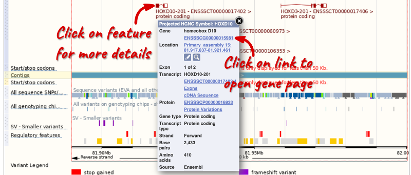
Searching for a gene
Another way to go to a gene of interest is to search directly for it.
We’re going to look at the NSDHL gene in Sus scrofa (Pig). From www.ensembl.org, select Pig from the drop-down menu in the blue box. Enter NSDHL into the search box and click the Go button.

Your search results include hits in all available Pig genomes. You can filter your results by breed in the left-hand panel. We want to restrict our results to entries in the Pig reference only. Under Restrict breeds to: in the left, click on Pig reference.
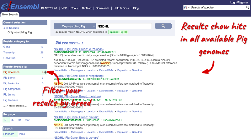
In your filtered search results, click on NSDHL (Pig Gene, Breed: reference) or the Ensembl ID ENSSSCG00005019191 to open the Gene tab:

Viewing the gene sequence
Let’s walk through some of the links in the left hand navigation column. How can we view the genomic sequence? Click Sequence in the left-hand panel.
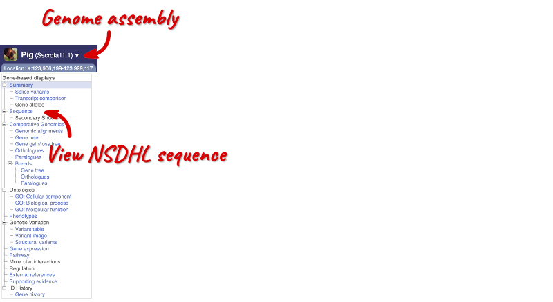

The sequence is shown in FASTA format. Take a look at the FASTA header:
>primary_assembly:Sscrofa11.1:X:123905599:123929717:1
The FASTA header always starts with a > followed by sequence information. Broken down, the information in the FASTA header is as follows:
>[primary_assembly:Sscrofa11.1]:[X]:[123905599]:[123929717]:[1]
- [primary_assembly:Sscrofa11.1] = name of the genome assembly
- = chromosome
- [123905599] = start coordinate
- [123929717] = end coordinate
- [1] = forward strand (-1 refers to reverse strand)
Exons are highlighted in orange within the genomic sequence. Variants can be added with the Configure this page button found in the left-hand panel. Click on the button to open a pop-up menu. Add the options Show variants: Yes and show links and Line numbering: Relative to this sequence.
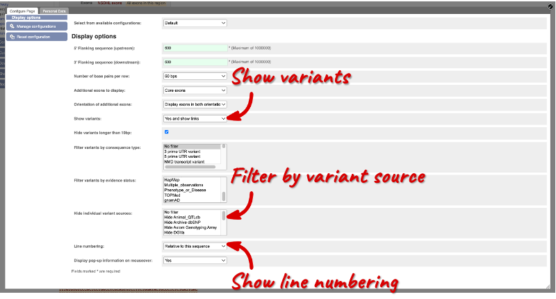
Save and close the pop-up menu by clicking on the check icon in the top right-hand corner.
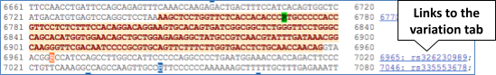
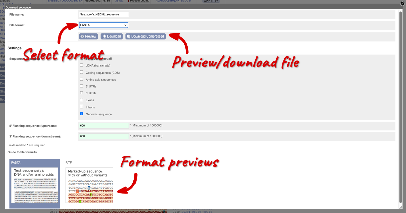
You can download this sequence by clicking in the Download sequence button  found above the sequence.
This will open a pop-up menu that allows you to pick the sequence format. You can download the sequence in plain FASTA or richt-text format (RTF), which includes all the coloured annotations and can be opened in a word processor. This button is available for all sequence views.
Viewing the gene function
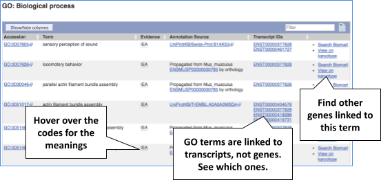
To find out what the protein does, have a look at Gene Ontology (GO) terms from the Gene Ontology consortium. There are three categories of GO terms:
- Biological process (what the protein does)
- Cellular component (where the protein is)
- Molecular function (how it does it)
Click on GO: Biological process in the left-hand panel to view GO terms associated with NSDHL.
Viewing gene information in external databases
Can our gene be found in other databases? Click on External references in the left-hand menu.
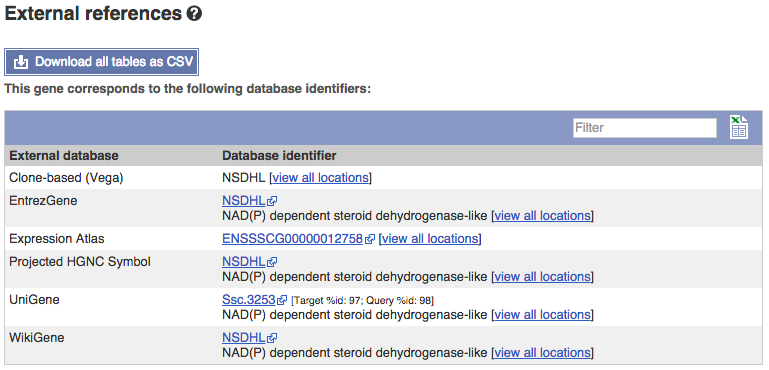
This page contains corresponding links to the gene in other projects, such as NCBI gene (formerly Entrezgene), Reactome gene and UniProtKB.
Demo: The Transcript tab
Let’s now explore one transcript/isoform/splice variant. Click on the Show transcript table button ![]() at the top of the page.
at the top of the page.
Have a look at the largest one, NSDHL-201.
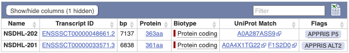
If we were to only choose one transcript to analyse, we would choose this one because it has the Ensembl Canonical flag. The Ensembl canonical transcript is a single, representative transcript identified at every locus. You can read more about canonical transcripts in the Genebuild documentation page.
Click on the transcript ID ENSSSCT00000048661.3 to open the corresponding to view more information. This opens the corresponding Transcript tab. The left-hand menu provides several options for the transcript NSDHL-201. You can find any protein-related information in the Transcript tab, if the transcript is protein-coding.
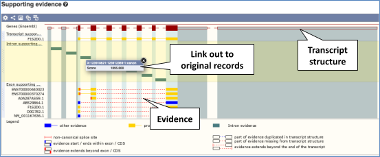
Transcript evidence
For detailed information on the support for this transcript, click on Supporting evidence.
Viewing the transcript sequence
Exon sequence
Click on Sequence: Exons in the left-hand panel.
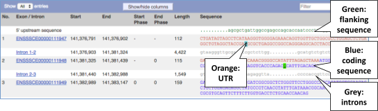
You may want to change the display (for example, to show more flanking sequence, or to show full introns). In order to do so click on the Configure this page button in the left-hand panel and change the display options accordingly.

cDNA sequence
Click on Sequence: cDNA in the left-hand panel to see the spliced transcript sequence.
UnTranslated Regions (UTRs) are highlighted in dark yellow, codons are highlighted in alternating white and light yellow, and exon sequences are shown in alternating black and blue colours (highlighting where another exon begins). Variants are represented by highlighted nucleotides and clickable IUPAC ambiguity codes representing the variation above the sequence.
Protein information
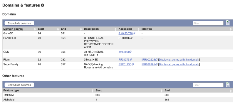
Click on Protein Information: Protein summary to view domains from Pfam, Superfamily, AlphaFold DB, and more.

Clicking on Domains & features shows a table of this information.
Transcript information in external databases
Click on External References: General identifiers in the left-hand panel. This page shows corresponding information in other databases such as the European Nucleotide Archive (ENA), UniProtKB and Reactome.

Exploring the Sus scrofa (Pig) TRAF3 gene
- Find the TRAF3 (TNF receptor associated factor 3) gene in the pig reference, and go to the Gene tab.
- Which strand of the genome is this gene located?
- How many transcripts are there of the gene?
- Which transcript produces the longest protein and how long is the protein sequence?
-
What are some functions of TRAF3 according to the gene ontology (GO)? Have a look at the Ontologies pages for this gene.
- In the transcript table, click on the transcript ID for TRAF3-201, and to open the corresponding Transcript tab.
- How many exons does it have?
- Are any of the exons completely or partially untranslated?
- Is there an associated sequence in UniProt? Have a look at the General identifiers for this transcript.
-
Are there microarray (oligo) probes that can be used to monitor the expression of TRAF3-201?
- Now find the TRAF3 gene in the Berkshire pig breed.
- Which strand of the genome is this gene located?
- How many transcripts are there of the gene?
- Which transcript produces the longest protein and how long is the protein sequence?
- How do the Ensmebl canonical transcripts differ between the pig reference and the Berkshire breed?
- Go to the Ensembl homepage. Select Pig from the drop-down list in the blue box, enter TRAF3 into the text box and click Go. In the search results page, click on Pig reference in the left-hand panel to restrict your results to the pig reference only. Click on the first hit TRAF3 (Pig Gene, Breed: reference) to open the Gene tab. Look at the Location section in the gene summary at the top of the page.
The TRAF3 gene is located on the forward strand.
Now look at the About this gene section in the gene summary at the top of the page.
TRAF3 has 4 transcripts.
Click on the Show transcript table button underneath the gene summary. Focus on the Protein column in the transcript table.
The transcript ENSSSCT00000101908.1 (TRAF3-201) produces the longest protein at 573 amino acid residues in length.
- Gene Ontology maps terms to a protein in three classes: biological process, cellular component, and molecular function.
Some of the GO terms associated to the TRAF3 gene are: regulation of cytokine production and proteolysis (biological process), protein kinase and metal ion binding (molecular function), and cytoplasm and endosome (cellular component).
- Click on ENSSSCT00000101908.1 in the transcript table. Under the summary information at the top of the page, focus on the About this transcript section.
This transcript has 11 exons.
Click on the Exons link in the left-hand side menu. In the Sequence column of the Exon table, look for any UnTranslated Regions (UTRs) which coloured in orange.
Only exon 11 is partially untranslated. You can also see this in the cDNA view if you click on Sequence: cDNA in the left-hand menu.
Click on External References: General identifiers in the left-hand menu. Look for UniProtKB in the External database column.
A0A4X1TTD0.19 and A0A8W4FAU5.6 from UniProt match the translation of the Ensembl transcript. Click on the IDs to open the corresponding entry in UniProt.
- In the left-hand menu, look for External References: Oligo probes.
The link is greyed out, which means that no commercial oligo probes are available to monitor expression of this transcript.
- Go to the Ensembl homepage by clicking on the Ensembl logo in the top left-hand corner of any page. Select Pig from the drop-down list in the blue box, enter TRAF3 into the text box and click Go. In the search results page, click on Pig berkshire in the left-hand panel to restrict your results to the Berkshire breed only. Click on the first hit TRAF3 (Pig Gene, Breed: berkshire) to open the Gene tab. Look at the Location section in the gene summary at the top of the page.
The TRAF3 gene is located on the forward strand in the Berkshire breed.
Now look at the About this gene section in the gene summary at the top of the page.
TRAF3 has 5 transcripts in the Berkshire breed.
Click on the Show transcript table button underneath the gene summary. Focus on the Protein column in the transcript table.
The transcript ENSSSCT00065038580.1 (TRAF3-205) produces the longest protein at 573 amino acid residues in length.
- The Ensembl canonical transcript in the pig reference genome is 6,677 bases in length. The Ensembl canonical transcript in the Berkshire breed is 6,340 bases in length. This suggests that the TRAF3 Ensembl canonical transcript in the reference has more/larger UTRs compared to the Berkshire breed. To compare, you can open the Sequence: Exons pages in the Transcript tab in both breeds and look at the length of the UTR (coloured in orange).
Exploring the MYH9 gene in Gallus gallus (Chicken)
- Find the MYH9 (myosin, heavy chain 9, non-muscle) gene in the chicken reference, and go to the Gene tab.
- On which chromosome and which strand of the genome is this gene located?
- Which transcript produces the longest protein and how long is the protein sequence?
-
What are some functions of MYH9 according to the Gene Ontology consortium? Have a look at the GO pages for this gene.
- In the transcript table, click on the transcript ID for MYH9-209, and go to the Transcript tab.
- How many exons does it have?
- Are any of the exons completely or partially untranslated?
- Is there an associated sequence in UniProt? Have a look at the General identifiers for this transcript.
- Are there microarray (oligo) probes that can be used to monitor ENSGALT00010036169.1 expression?
- Go to the Ensembl homepage. Select Chicken from the drop-down list in the blue box, enter MYH9 and click Go. In the search results page, click on Chicken reference in the left-hand panel to restrict your results to the reference genome only. Click on the first hit MYH9 (Chicken Gene, Breed: reference) to open the Gene tab. Look at the Location section in the gene summary at the top of the page.
The gene is located on chromosome 1 on the forward strand.
Now click on the Show transcript table button and focus on the Protein column in the Transcript table.
The transcript ENSGALT00010036169.1 (MYH9-209) produces the longest protein at 1,960 amino acid residues.
- Gene Ontology maps terms to a protein in three classes: biological process, cellular component, and molecular function.
Meiotic spindle organisation, cell morphogenesis, and angiogenesis are some of the roles associated with the MYH9 gene.
- Click on ENSGALT00010036169.1 in the Transcript table to open the corresponding Transcript tab. Look at the About this transcript section in the transcript summary at the top of the page.
The transcript has 41 exons.
Click on the Exons link in the left-hand side menu. In the Sequence column of the Exon table, look for any UnTranslated Regions (UTRs) which coloured in orange.
Exon 1 is completely untranslated, and exons 2 and 41 are partially untranslated. You can also see this in the cDNA view if you click on Sequence: cDNA in the left-hand menu.
Click on External References: General identifiers in the left-hand menu. Look for UniProtKB in the External database column.
A0A1D5PM19.34 from UniProt matches the translation of the Ensembl transcript. Click on A0A1D5PM19.34 to open the corresponding UniProt entry in a new browser tab.
- In the left-hand menu, look for External References: Oligo probes.
There are probes from Affy and Agilent that can be used to monitor expression of this transcript.
Exploring a Triticum aestivum (Wheat) gene
Start in the Ensembl Plants homepage and select the Triticum aestivum IWGSC genome to answer the following questions:
-
What GO: Molecular function terms are associated with the Wheat gene TraesCS6D02G180200?
-
Go to the transcript tab. How many exons does it have? Which one is the longest? Approximately, how much of that is coding?
-
What domains can be found in the protein product of this transcript? What prediction method(s) identified these domains?
- Go to Ensembl Plants, select Triticum aestivum from the drop down menu then type
TraesCS6D02G180200into the search box. Click on the gene name link TraesCS6D02G180200 in the search results. Click on GO: Molecular function in the left-hand menu.There is one term listed: GO:0005515, protein binding.
- Click on the transcript tab at the top of the page. Click on Exons in the left-hand menu.
There are six exons. Exon 6 is longest with 485 bp, of which around one sixth is coding.
- Click on either Protein Summary or Domains & features in the left-hand menu to view the data graphically or as a table, respectively.
Leucine-rich repeats are predicted by many different methods, however each method predict the leucine-rich repeats at different positions.
Comparative genomics
Demo: comparative genomics
Gene tab: homologues and gene trees
Homologues across different species
Let’s explore homologues of the BRCA2 gene in the pig (Sscrofa11.1) reference genome. Search for the gene and go to the Gene tab. Homologues can be found under Comparative Genomics in the left-hand menu. If there are no orthologues or paralogues, the option will be greyed out. Paralogues is greyed out for BRCA2 indicating that there are no paralogues. Click on Comparative Genomics: Orthologues to see the available orthologues. Select the species set Laurasiatheria to show carnivores, ungulates and insectivores only in the Orthologue table at the bottom.
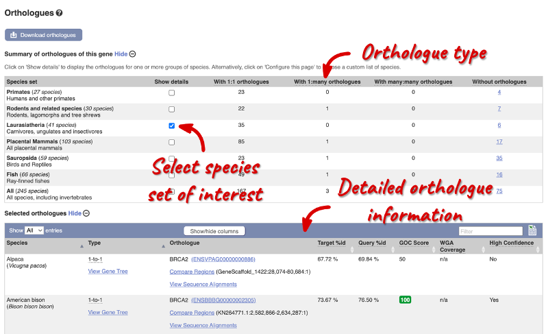
Let’s look at the Cow orthologue.
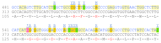
Links from the orthologue allow you to view alignments of the orthologous proteins and cDNAs. In the table, click on View Sequence Alignments under the Orthologue header and then click on View Protein Alignment in the pop-up menu.
Homologues across different pig breeds and other livestock species
Let’s explore homologues of the BRCA2 gene across different pig breeds and other livestock species. Click on Comparative Genomics: Breeds: Orthologues to see the available orthologues. In the table, use the filter in the top right-hand corner and enter *Pig. This filters the table to include only pig breeds.
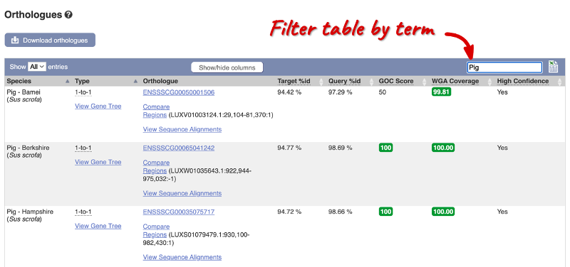
Let’s look at the Pig - Hampshire orthologue.
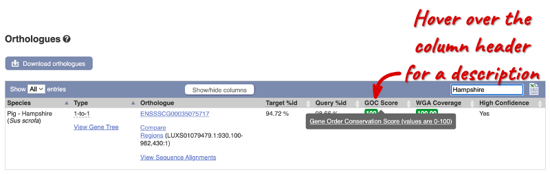
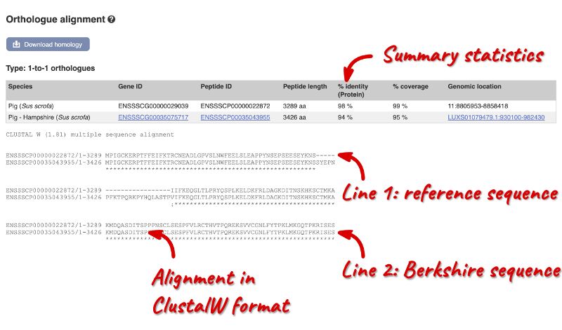
Links from the orthologue allow you to view alignments of the orthologous proteins and cDNAs. In the table, click on View Sequence Alignments under the Orthologue header and then click on View Protein Alignment in the pop-up menu.
Gene trees across different species
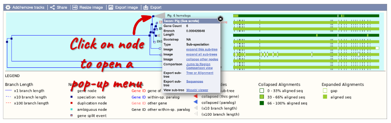
Click on Comparative Genomics: Gene tree to display the current gene in the context of a phylogenetic tree used to determine orthologues and paralogues.
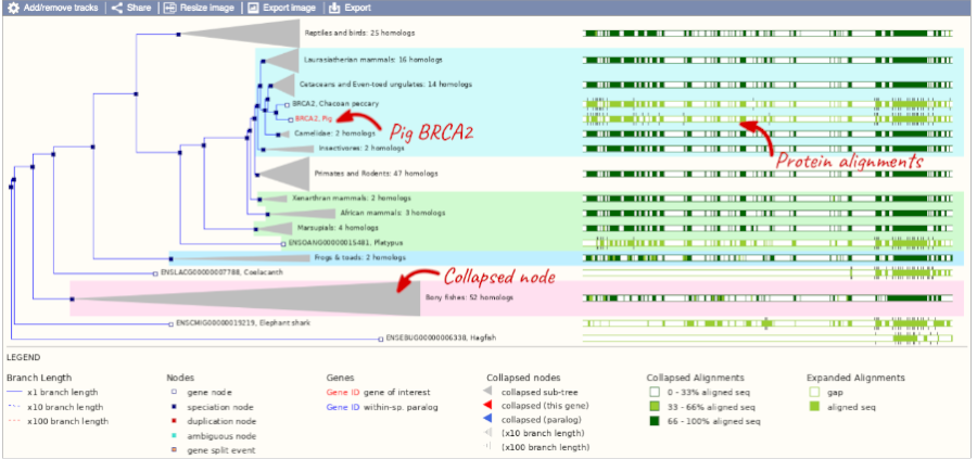
You can change the gene tree display by using the View options below the image or the Configure this page button on the left-hand panel. You can also click on the individual nodes in the phylogeny to open a pop-up menu for other display options. Grey funnels indicate collapsed nodes. You can expand them by clicking on the node and selecting expand this sub-tree from the pop-up menu.
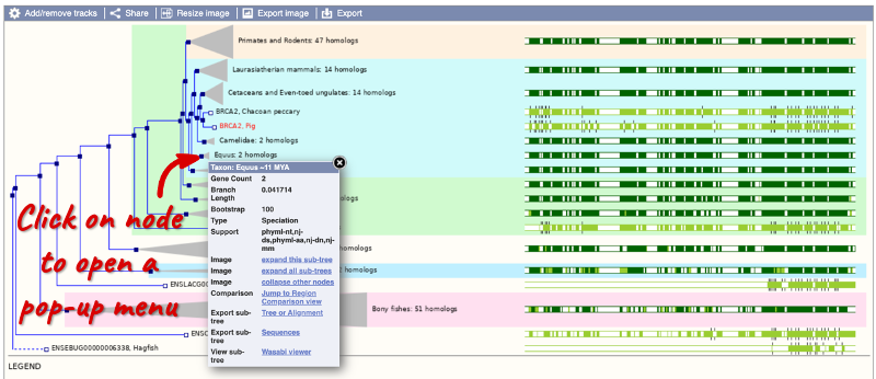
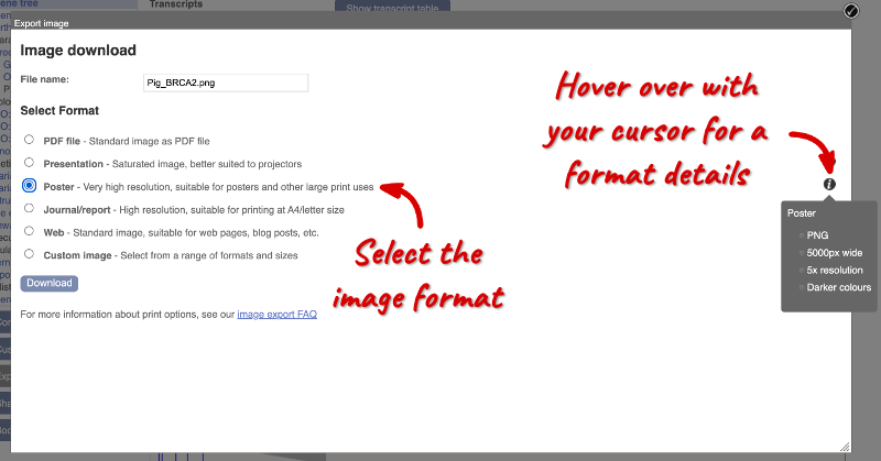
You can download the tree in a variety of formats. Click on the Export image button above the phylogeny to download the image in various formats.
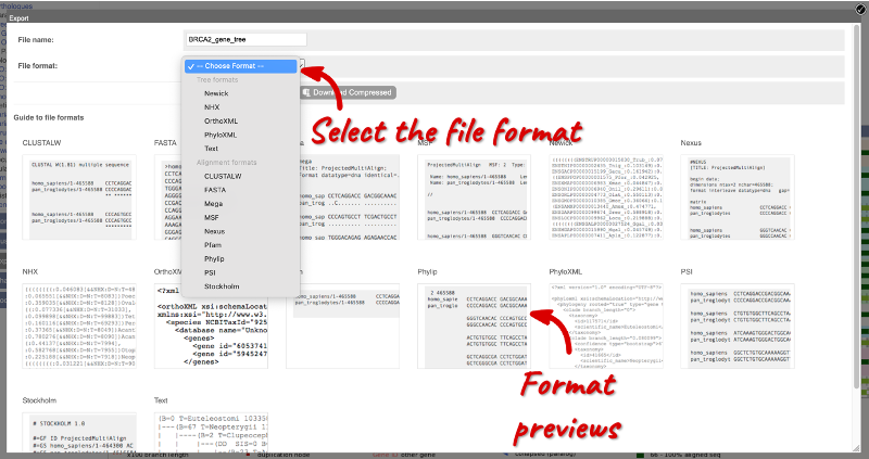
Click on the Export button above the phylogeny to download the phylogeny or alignments in various formats.
Gene trees across different pig breeds and other livestock species
Click on Comparative Genomics: Breeds: Gene tree to display the current gene in the context of a phylogenetic tree across different pig breeds and other livestock species.
You can change the gene tree display by using the View options below the image or the Configure this page button on the left-hand panel. You can also click on the individual nodes in the phylogeny to open a pop-up menu for other display options. Grey funnels indicate collapsed nodes. You can expand them by clicking on the node and selecting expand this sub-tree from the pop-up menu.
Location tab: alignments and synteny
Pairwise and multiple whole-genome alignemnts
Conservation scores and constrained elements
Let’s look at some of the comparative genomics views in the Location tab. Go to the region 15:81873000-82000800 in the pig (Sscrofa11.1) reference genome. This region contains the HoxD cluster which is involved in limb development and is highly conserved between species.
You can turn on Genomic Evolutionary Rate Profiling (GERP) conservation scores and constrained elements. GERP scores assess the conservation of genomic elements across species. Positive scores represent highly-conserved regions in the genome (which suggest critical functional regions in the genome), while negative scores represent highly-variable regions. Constrained elements highlight these highly conserved regions. You can read more about conservation scores and constrained elements in the Ensembl comparative genomics documentation.
Click on the Configure this page button in the left-hand panel. In the pop-up menu, go to Comparative genomics: Conservation regions in the left-hand panel and turn on the tracks for Constrained elements for 16 pig breeds EPO-Extended and Conservation score for 16 pig breeds EPO-Extended on the right. Save and close the menu.
You can now see the conservation scores in pale pink. These were used to determine the peaks indicated in the constrained elements track in dark pink. This track indicates regions of high conservation between species, considered to be “constrained” by evolution.
Pairwise whole-genome alignments
Let’s look at individual species comparative genomics tracks. Click on the Configure this page buton . In the pop-up menu, go to Comparative genomics: BLASTz/LASTz alignments in the left-hand menu. Here, you can enable alignments between closely related species. Let’s visualise genomic alignments of species with differing relatedness to the pig reference:
- Pig - Largewhite (Sus scrofa) - LASTz net
- Chacoan peccary (Catagonus wagneri) - LASTz net
- Human (Homo sapiens) - LASTz net
Save and close the menu.

From the alignment, we can see that the most distantly related species (Human) has the largest number of gaps in the alignment. If you compare the alignment region that contains a lot of gaps (marked above) with the 16 way GERP elements track, you’ll notice that this region does have any constrained elements, and therefore suggests that the genomic sequence is highly variable across species.
We can also look at the sequence alignment itself. Click on Alignments (text) in the left-hand panel. Click on Select another alignment and add Pig - Largewhite in the pop-up menu. Click Apply to save and close the menu.
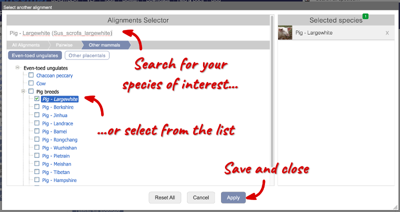
You will see a list of the regions aligned, followed by the sequence alignment. Exons are shown in red.
To compare with both contigs visually, go to Comparative Genomics: Region Comparison in the left-hand menu.
To add a species to this view, click on the blue Select species or regions button. Choose Pig - Largewhite from the list then close the menu.

You can configure this view for both species. Click on Configure this page and look in the top left of the menu.
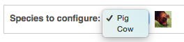
The drop down allows you to configure each species separately.
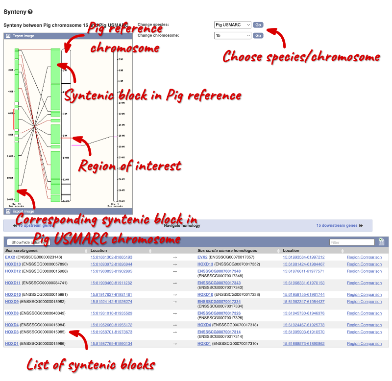
Synteny
Synteny describes the conserved order of genes in a sequence alignment between two species. We can view large-scale syntenic regions from our chromosome of interest. Click on Comparative Genomics: Synteny in the left-hand menu.
Multiple whole-genome alignments
Gene trees and homologues in Sus scrofa (Pig) breeds
We are going to look at the PLAG1 gene in the pig reference (Sscrofa11.1) genome and explore its gene tree and homologues.
-
Have orthologues been identified in any pig breeds? If so, which ones?
-
Open the cDNA sequence alignment against the Tibetan breed. What does the asterisk (*) symbol mean in the alignment? What is the % identity (cDNA) and what does the number stand for?
-
Let’s look at the PLAG1 breed gene tree. How many genes are depicted in the gene tree? According to the gene tree, which orthologue is the most closely related to the pig reference PLAG1 gene? What is the Ensembl ID of the orthologue and what strand is it located on?
-
Export the gene tree in Newick format.
- Open the Gene tab for the PLAG1 gene (ENSSSCG00000006247) in the pig reference (Sscrofa11.1) genome. In the left-hand panel, click on Comparative Genomics: Breeds: Orthologues to explore orthologues in pig breeds.
PLAG1 orthologues have been identified in all 12 available pig breeds: Bamei, Berkshire, Hampshire, Jinhua, Large white, Meishan, Pietrain, Rongchang, Tibetan, Wuzhishan and USMARC.
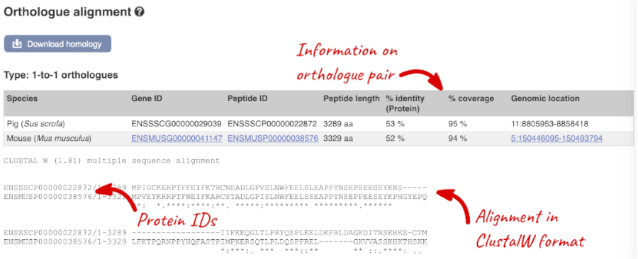
- Stay in the Comparative Genomics: Breeds: Orthologues page and look for the Pig - Tibetan entry in the Orthologues table. Click on View Sequence Alignments and select View cDNA Alignment in the pop-up menu. This will lead you to the sequence alignment between the pig reference PLAG1 gene and the orthologue in the Tibetan breed. Click on the ? icon above the alignment to open the corresponding help page and find a description of the data (including descriptions of the conservation codes and summary statistics).
The alignment is in ClustalW format and the asterisk (*) is a conservation code that denotes the aligned nucleotides are identical in both sequences.
In the **Type: 1-to-1 orthologues table, look for the column **% identity (cDNA).
The % identity (cDNA) describes the number of identical nucleotides between the two sequences in the alignment. The % identity (cDNA) between the pig reference and the Tibetan breed is 99%, meaning 99% of the cDNA sequence alignment is identical.
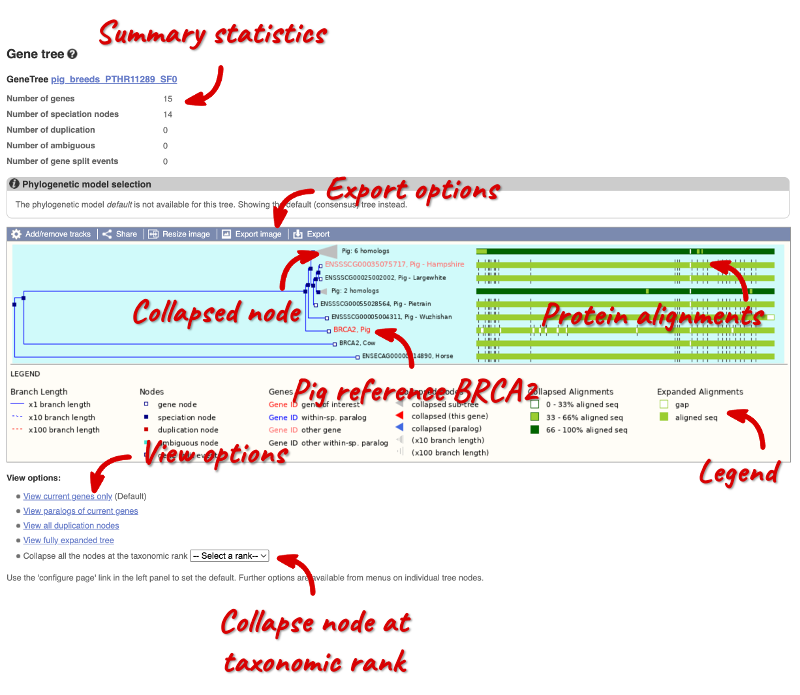
- In the left-hand panel, click on Comparative Genomics: Breeds: Gene tree. Above the gene tree image, you can find some summary statistics.
There are 16 genes in the gene tree.
In the gene tree, look for PLAG1, Pig (coloured in red) in the tree and find the closest branch.
The most closely related orthologue is the PLAG1 gene in the Berkshire breed. Clicking on PLAG1, Pig - Berkshire opens more details on the orthologue including the Ensembl ID (ENSSSCG00065079212) and strand (reverse).
- Click on the Export button at the top of the gene tree image. In the pop-up menu, select File format: Newick (you can find a preview of each file format underneath) and Preview the file on your browser.
Whole-genome alignments in Sus scrofa (Pig)
Go to www.ensembl.org to find the DBH gene on the reference pig genome (Sscrofa11.1).
-
Go to the Location page for this gene. View the Alignments (image) and Alignments (text) for the 16 pig breeds EPO-Extended. Do all the pig breeds show a gene in these alignments?
-
Export the alignments in ClustalW format.
-
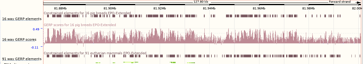
Go to the Region in detail view and turn on the 16 pig breeds EPO-Extended multiple alignment, conservation score and constrained elements tracks. Are there any differences between the conservation score and constrained elements tracks?
-
Compare the 16 way GERP elements track and the 91 way GERP elements track that is already turned on by default.
- What is the difference between the two tracks?
- Which regions of the gene do most of the constrained element blocks match-up to?
- How can you find more information on how the constrained elements track was generated?
- Search for the DBH(ENSSSCG00000005742) gene in the Pig (SScrofa11.1) reference and switch to the Location tab. Click on Alignments (image) in the left-hand panel. Under Alignment, click on the Select alignment button to open a pop-up menu. Enable the 16 pig breeds EPO-Extended alignment, then close the menu.
All 12 big breeds as well as cow, horse and sheep have an alignment at this region. This can also be seen in the Alignments (text) page, where the exons are coloured in red.
-
You can export the alignments from either the Alignments (images) or Alignments (text) pages. Click on the blue Download alignments button at the top of the page. From the pop-up menu, select File format: CLUSTALW. You can Preview the alignment in a new browser tab, or Download the file to your local machine.
- Click on Region in detail in the left-hand panel. In the pop-up menu, go to the Comparative genomics section and turn on the following tracks:
- Multiple alignments: 16 pig breeds EPO-Extended
- Conservation score for 16 pig breeds EPO-Extended
- Constrained elements for 16 pig breeds EPO-Extended
Close the pop-up menu and find the tracks in the Region in detail view.
The 16 pig breeds EPO-extended track shows that the entire region for the DBH gene can be aligned among the big breeds and related agricultural species. The Constrained elements and Conservation score tracks show where the conserved sequence is located in the alignment. Regions where constrained elements are found are regions with high GERP scores. Higher conservation regions (i.e. constrained elements) match up with exonic regions (exons tend to be highly conserved) of the gene. Note that there are intronic regions that seem to be fairly conserved across the species available.
- For both 16 way GERP elements and 91 way GERP elements tracks, click on the track name to open the pop-up menu. Hover over the i icon with your cursor to find a track description.
The 16 way GERP elements track shows the 16 pig breeds EPO-Extended multiple whole-genome alignment. The 91 way GERP elements track shows the 91 eutherian mammals EPO-Extended multiple whole-genome alignment.
You can move the 91 way GERP elements track closer to the 16 way GERP elements track to make any comparisons easier.
You will notice that constrained elements match-up with exonic regions in the genome.
Click on the track name and open the information tab in the pop-up menu. Click on the GERP conservation score link.
This opens the documentation page for the multiple whole-genome alignment calculations.
Orthologues and gene trees for the Gallus gallus (Chicken) BRAF gene
- Let’s explore the orthologues of the chicken BRAF gene.
- How many orthologues are predicted for the chicken BRAF in sauropsida (birds and reptiles)?
- How much sequence identity does the Anolis carolinensis (Green anole) protein have to the chicken one?
- Export the protein alignment in Clustal format.
- Look at the orthologue in human. Is there a genomic alignment between human and chicken? Is there a gene for both species in this region?
- Go to the Ensembl homepage, select Chicken from the drop-down list in the blue search box, enter BRAF and click Go. Open the **Gene tab and click on Comparative Genomics: Orthologues at the left-hand panel to see all the orthologous genes.
There 25x 1:1 and 1x 1:many orthologues in sauropsida.
Find Green anole in the Selected orthologues (you can use the filter in the top right-hand corner).
The percentage of identical amino acids in the Green anole protein (the orthologue) compared with the gene of interest. i.e. chicken BRAF (the target species/gene) is 84.42%. This is known as the Target %id. The identity of the gene of interest (chicken BRAF) when compared with the orthologue (Green anole BRAF, the query species/gene) is 94.67% (this is the Query %id).
Click on the View Sequence Alignments link in the Orthologue column of the Selected orthologues table and select View Protein Alignment in the pop-up menu. To download the alignment, click on the Download homology button and select the CLUSTALW file format in the pop-up menu.
- Click on Comparative Genomics: Genomic alignments in the left-hand panel. Click on Select an alignment and add Human in the pop-up menu. In the table, select Block 1 to view the largest block of aligned sequence (this will lead you to the Location tab). Click on Display full alignment. In the alignment, sequences coloured in red are exons.
There is a gene in both species in this region. You can find where the start and stop codons are located if you Configure this page and select Codons: START/STOP codons in the options.
Note: You can visualise the alignment in the genomic context in the Comparative Genomics: Region Comparison page (blue lines connect homologous genes between species). Go to Select species or regions, add Human and close the pop-up menu. Click on Configure this page. In the pop-up menu under Comparative features category, enable the Join genes option. You may need to zoom out on the Region in detail view to see blue lines connecting all the homologous genes between chicken and human genes in that region.
Homologues and gene trees for the Triticum aestivum (wheat) RHT1 gene
Go to Ensembl Plants and answer the following questions:
-
How many orthologues are predicted for the Triticum aestivum (wheat) gene RHT1 (gene ID TraesCS4D02G040400) gene in Liliopsida?
-
How much sequence identity does the Secale cereale (rye) protein have to the maize one?
-
Download the alignment in Nexus format.
-
Open the gene tree for the wheat RHT1 gene. What is the gene tree ID?
-
How many speciation and duplication nodes does the phylogeny have?
Go to the Ensembl Plants homepage, select Triticum aestivum from the Species drop-down and search for TraesCS4D02G040400. Click through to the Gene tab. On the Gene tab, click on Plant Compara: Orthologues at the left-hand side of the page to see all the orthologous genes.
- These are the orthologues in the Liliopsida:
- 24 1-to-1
- 9 1-to-many
- 0 many-to-many
- Filter the table by entering
Secale cerealein the filter box on the top right-hand corner of the table.The percentage of identical amino acids in the rye protein (the orthologue) compared with the gene of interest (i.e. wheat RHT1; the target species/gene) is 98.71%. This is known as the Target %ID. The identity of the gene of interest (wheat RHT1) when compared with the orthologue (the rye gene, i.e. the query species/gene) is 97.91% (the query %ID).
Note the differences in the values of the Target and Query % ID reflects the different protein lengths for the genes. -
Click on View Sequence Alignments in the Orthologue column. Select View Protein Alignment from the pop-up menu. Click on the green Download homology button above the table and select Nexus. Click on Download or Download Compressed to save the alignment on your local machine.
- Go to Plant Compara: Gene tree in the left-hand menu. You can find the gene tree ID above the phylogeny.
The gene tree ID is EPlGT00940000163877.
- You can find some summary statistics below the gene ID.
There are 418 speciation nodes and 149 duplication nodes.
Variation
In any of the sequence views shown in the Gene and Transcript tabs, you can view variants on the sequence. You can do this by clicking on Configure this page from any of these views.
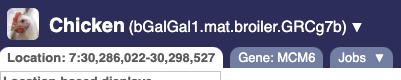
Let’s take a look at the Gene sequence view for MCM6 in chicken. Search for MCM6 and go to the Sequence view.
If you can’t see variants marked on this view, click on Configure this page and select Show variants: Yes and show links.
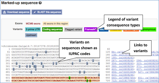
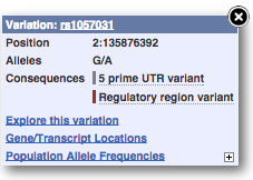
Find out more about a variant by clicking on it.
You can add variants to all other sequence views in the same way.
You can go to the Variation tab by clicking on the variant ID. For now, we’ll explore more ways of finding variants.
To view all the sequence variations in table form, click the Variant table link at the left of the gene tab.
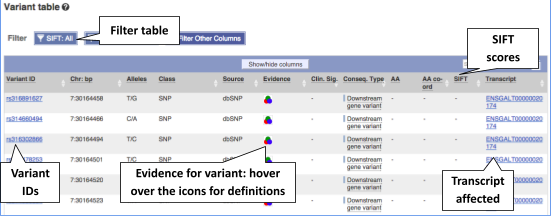
You can filter the table to only show the variants you’re interested in. For example, click on Consequences: All, then select the variant consequences you’re interested in.
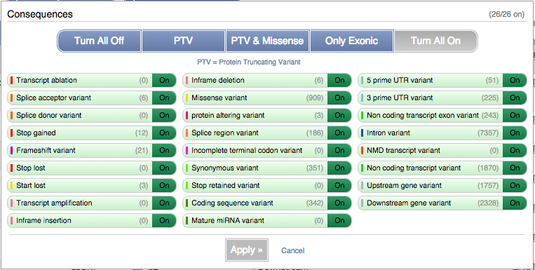
You can also filter by SIFT, or click on Filter other columns for filtering by other columns such as Evidence or Class.
The table contains lots of information about the variants. You can click on the IDs here to go to the Variation tab too.
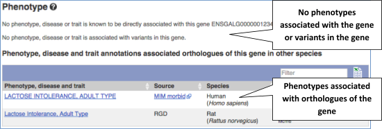
You can also see the phenotypes associated with a gene. Click on Phenotype in the left hand menu.
Let’s have a look at variants in the Location tab. Click on the Location tab in the top bar.
Click on Configure this page and open Variation from the left-hand menu.
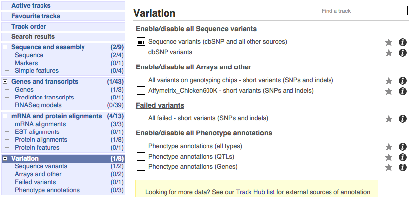
There are various options for turning on variants. You can turn on variants by source, by frequency, presence of a phenotype or by individual genome they were isolated from. You can also turn on QTLs, which cover a locus without being associated with a specific variant. Turn on the following variation tracks.
- All variants on genotyping chips - short variants (SNPs and indels)
- Phenotype annotations (QTLs)

Click on a variant to find out more information. It may be easier to see the individual variants if you zoom in.
Let’s have a look at a specific variant, which happens to fall within the MCM6 gene: rs14625781.
The easiest way to find this variant is if we put rs14625781 into the search box. Click through to open the Variation tab.
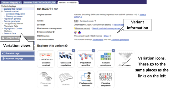
The icons show you what information is available for this variant. Click on Genes and regulation, or follow the link at the left.
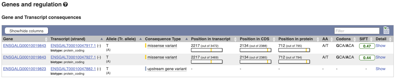
This variant is found in three transcripts of the MCM6 gene, and is missense in two. SIFT predicts that it is unlikely to affect protein function of either (Tolerated).
Let’s look at population genetics. Either click on Explore this variant in the left hand menu then click on the Population genetics icon, or click on Population genetics in the left-hand menu.
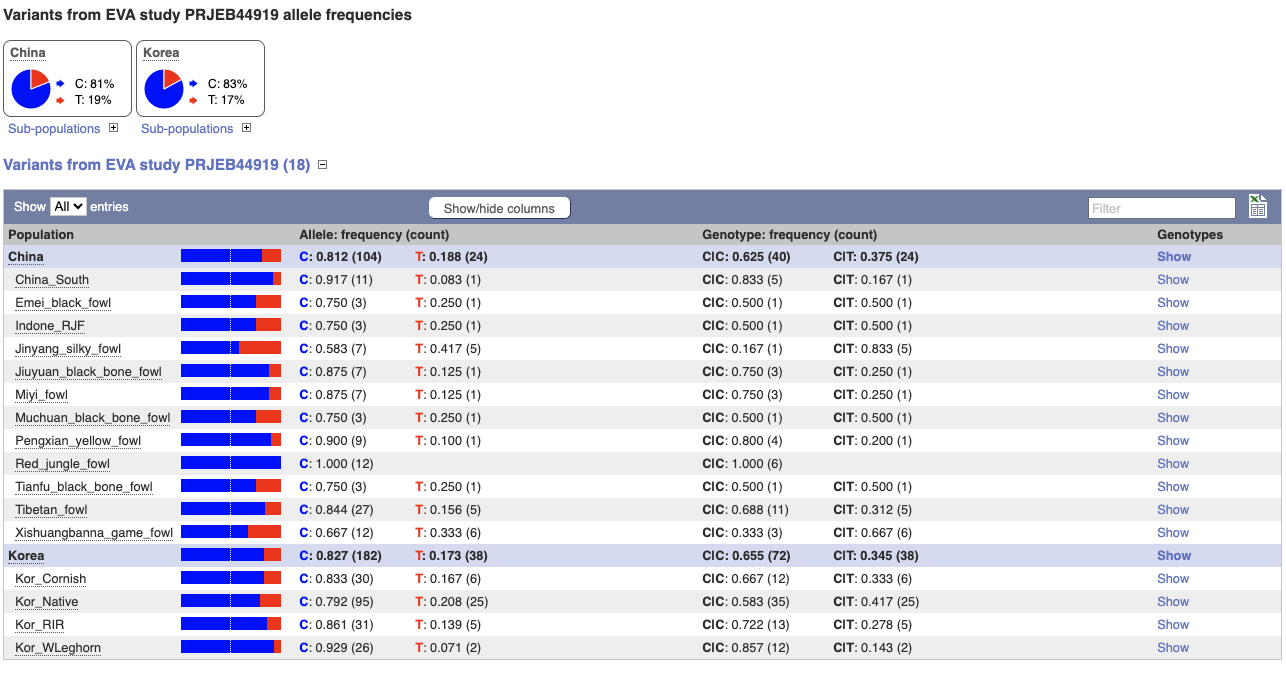
We can see data from EVA study PRJEB44919 showing the frequency of the alleles and genotypes. We can see what animals these genotypes were actually observed in by going to Sample genotypes.
Click on Phylogenetic context to see the variant in other species.
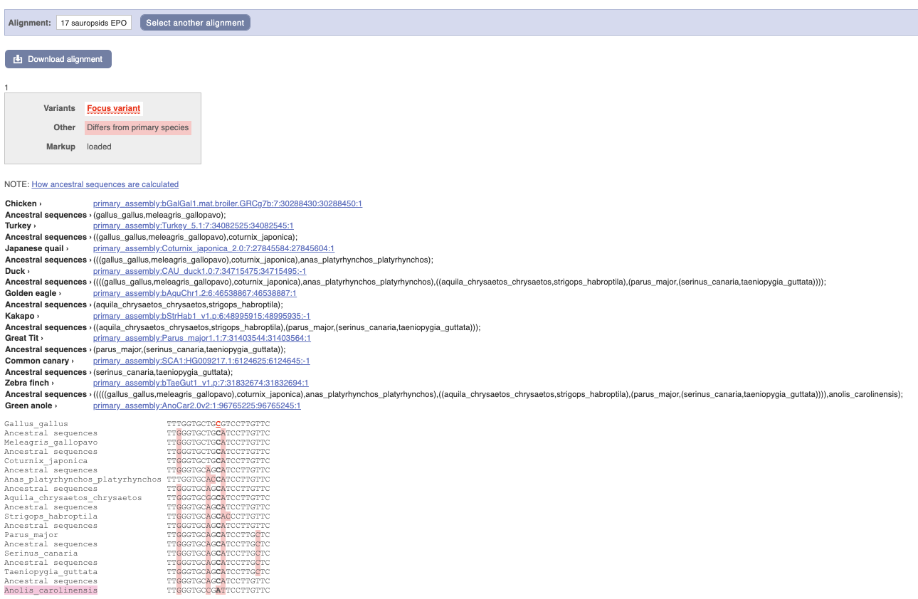
We can see that other birds also have the C alleles as a reference whereas Anolis_carolinensis has an A allele.
Exploring a SNP in chicken
(a) Find the page with information for the chicken SNP rs10731268.
(b) What gene(s) does rs10731268 fall within? What is its effect?
(c) Have any papers been written mentioning rs10731268? What are they about?
(d) What allele is at this position in other birds? What is the likely ancestral allele?
(a) Go to the Ensembl homepage.
Type rs10731268 in the Search box, then click Go. Click on rs10731268.
(b) Click on Genes and Regulation in the side menu (or the Genes and Regulation icon).
rs10731268 falls within 2 genes: ENSGALG00010028562 and ENSGALG00010028568 (HGNC: MLLT1). This variant has a missense consequence in seven transcripts of the ENSGALG00010028562 gene, and downstream gene variant consequence in three transcripts of the ENSGALG00010028568 (HGNC: MLLT1) gene.
(c) Click on Citations in the left hand side menu.
This variant is mentioned in the paper ‘Identification and characterization of genes that control fat deposition in chickens’ from 2013 by D’Andre et al. Click on the PubMed ID 24206759 to go to the paper.
(d) Click on Phylogenetic Context in the side menu. Select Alignment: 17 sauropsids EPO and click Go.
Japanese quail, Duck, Golden Eagle, Common canary and Zebra finch all have an A in this position. This suggests that A may be the ancestral allele.
Exploring a variant in pig
The human gene MC4R has been associated with obesity. The SNP rs81219178 has been identified as a variant in the pig MC4R gene.
(a) What is the amino acid change caused by rs81219178 in MC4R of the pig? Is the change likely to alter the protein function?
(b) How many transcripts does this variant affect? What are the consequences of this variant?
(a) Go to the Ensembl homepage.
Type rs81219178 in the Search box, then click Go.
Click on rs81219178 (Pig Variant, Breed: reference).
Click on Genes and regulation in the left-hand menu or on the icon.
The variant causes a D->N amino acid change (Aspartic acid -> Asparagine). The SIFT score of 0.01 predicts that this change will have a deleterious effect on the protein.
(b) This variant affects one transcript (ENSSSCT00000091644.1) of ENSSSCG00000051798 gene and it has the missense consequence.
Ensembl VEP
We have identified seven variants in pig:
rs319195925, rs80805426, rs81267388, rs80854621, rs711163915, rs321793337, rs792403417
We will use the Ensembl VEP to determine:
- If the variants have been annotated in Ensembl already
- If genes are affected by the variants
Go to the front page of Ensembl and click on Variant Effect Predictor in the Tools section or click on VEP in the top header.
This page contains information about the VEP, including a link for downloading the script version of the tool. Click on the Launch VEP button to open the input form.
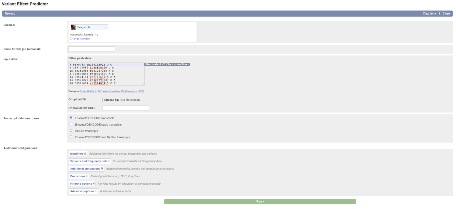
Lets input the variants data in VCF format:
Chromosome Position Name Reference Alternative
Put the following into the Input data box:
9 9580742 rs319195925 T C
1 213701082 rs80805426 C A
15 83361856 rs81267388 A G
1 159538854 rs80854621 A G
14 50574184 rs711163915 C A
14 50571223 rs321793337 G A
14 50571474 rs792403417 C T
The VEP will detect automatically that the data is in VCF format.
There are further options that you can choose for your output. These are categorised as Identifiers, Variants and frequency data, Additional annotation, Predictions, Filtering options and Advanced options. Let’s open all menus and take a look.
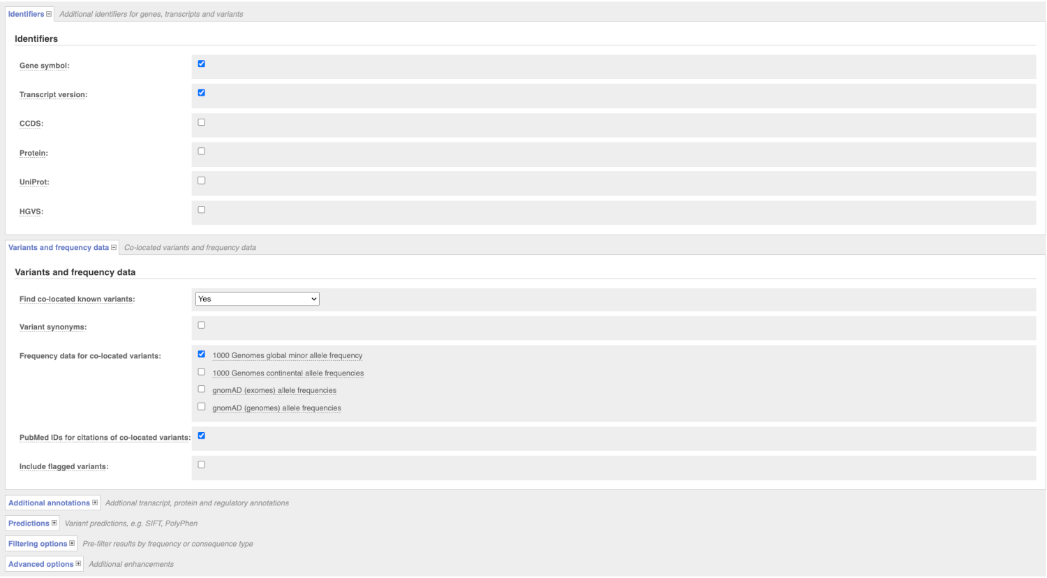
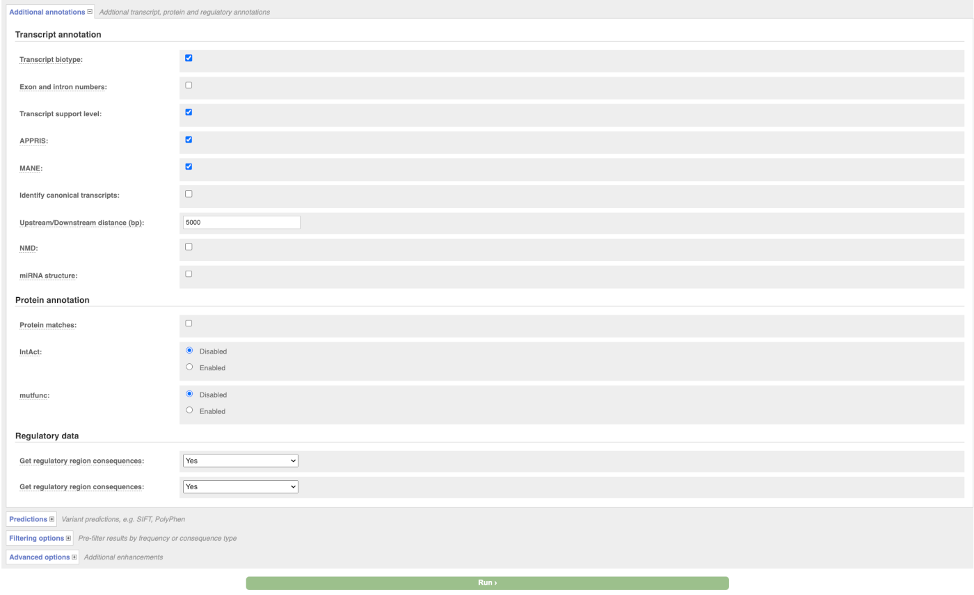
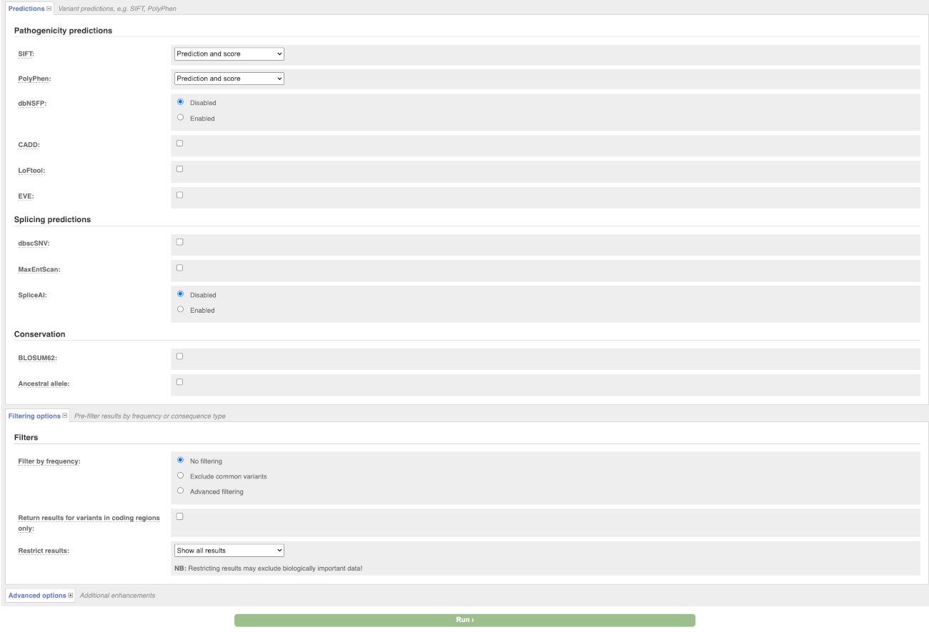
Hover over the options to see definitions.
When you have selected everything you need, scroll right to the bottom and click Run.
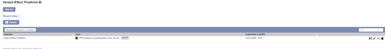
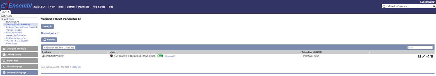
The display will show you the status of your job. It will say Queued, then automatically switch to Done when the job is done, you do not need to refresh the page. You can save, edit, share or delete your job at this time. If you have submitted multiple jobs, they will all appear here.
Click on View Results once your job is done.
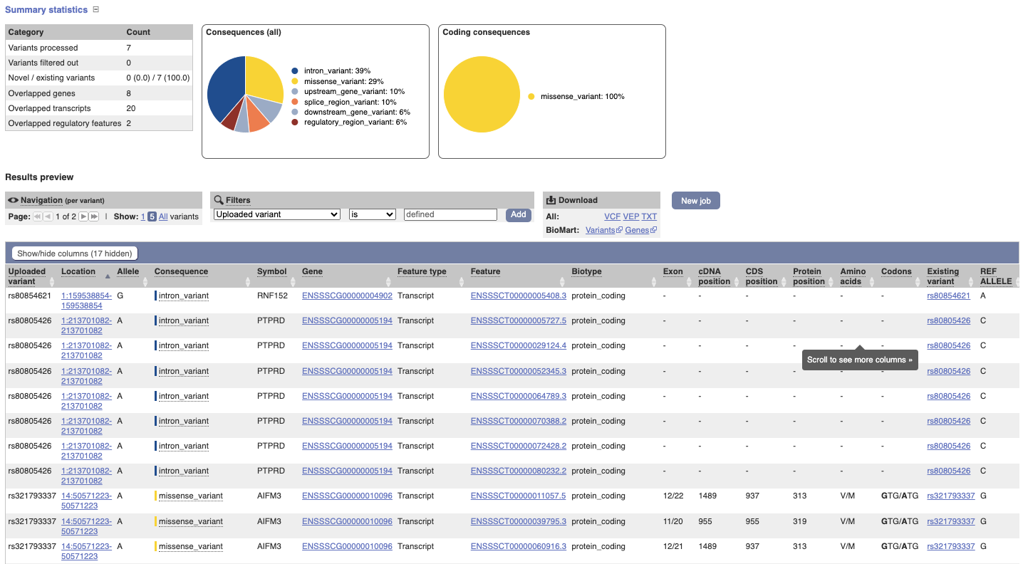
In your results you will see a graphical and table summary of the data as well as a table with the detailed results.
VEP for chicken data
We have identified a few variants associated with body size in chicken (bGalGal1.mat.broiler.GRCg7b):
chr 6, genomic coordinate 23650222, alleles A/C, forward strand
chr 6, genomic coordinate 23645685, alleles C/A, forward strand
chr 1, genomic coordinate 51237121, alleles C/T, forward strand
(a) Which genes and transcripts do these variants map to?
(b) What are the consequence terms for these variants?
(c) Which regulatory feature is affected by the variants?
Go to the Variant Effect Predictor (VEP) under Tools on the top banner of any Ensembl page.
Copy the following into the Paste data text box: 6 23650222 23650222 A/C + var1, 6 23645685 23645685 C/A + var2, 1 51237121 51237121 C/T + var3,
Note that this is the Ensembl default format (chr start end reference/alternate alleles). For additional formats accepted by VEP, have a look here: http://www.ensembl.org/info/docs/tools/vep/vep_formats.html
Click Run.
(a) In the Results table, you’ll see that the variants fall into three genes.
(b) The consequence terms are listed in the Consequence column and Consequences (all) chart and include intron_variant, regulatory_region_variant, upstream_gene_variant and downstream_gene_variant.
(c) Variant 3 at 1:51237121-51237121 with T allele affects regulatory feature ENSR00000006264 (promoter).