Filter Events by Year
Ensembl Plants Browser Workshop - CeniCafé
Course Details
- Lead Trainer
- Aleena Mushtaq
- Event Date
- 2024-07-04
- Location
- CeniCafé, Pereira, Colombia
- Description
- Work with the Ensembl Outreach team to get to grips with the Ensembl Plants browser, accessing gene, regulation and comparative genomics data.
- Survey
- Ensembl Plants Browser Workshop - CeniCafé Feedback Survey
Demos and exercises
Ensembl species
Demo: Introduction to Ensembl Plants
Homepage
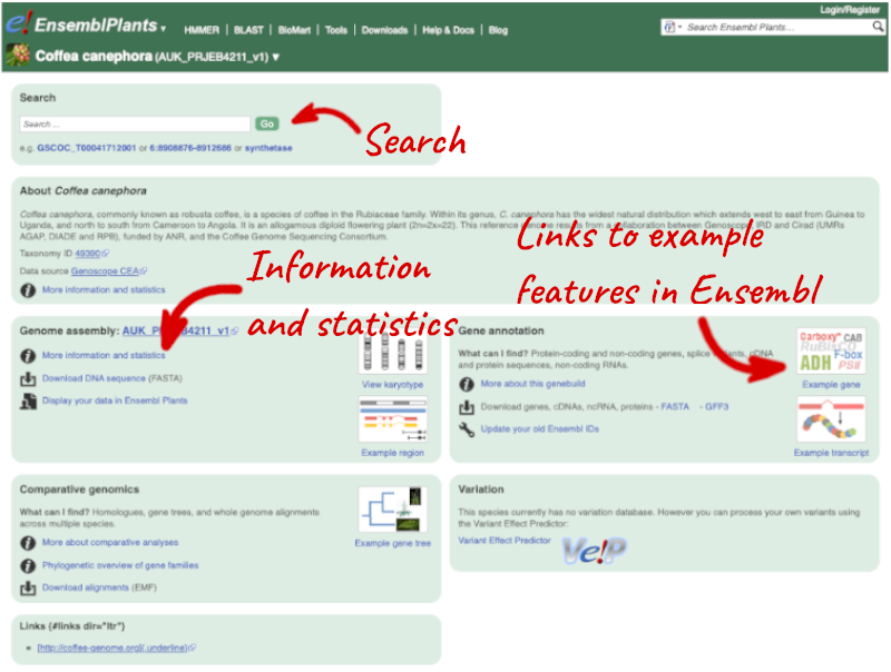
The front page of Ensembl Plants is found at plants.ensembl.org. It contains lots of information and links to help you navigate Ensembl Plants:
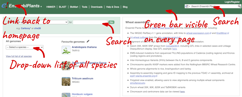
At the top left you can see the current release number and what has come out in this release.
Available species
Click on View full list of all species.
Click on the scientific name of your species of interest to go to the species homepage. We’ll click on Coffea canephora.
Species information
Here you can see links to example pages and to download flatfiles. To find out more about the genome assembly and genebuild, click on More information and statistics.
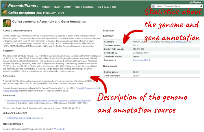
Here you’ll find a detailed description of how the genome was produced and links to the original source. You will also see details of how the genes were annotated.
Exploring the Coffee genome assembly
-
What is the name of the coffee variety represented in Ensembl?
-
Who produced this genome assembly and annotation?
-
What is the length of the Coffea canephora genome assembly? How many coding genes are annotated across the genome?
Select Coffea canephora from the drop down species list, or click on View full list of all species, then choose Coffea canephora from the list to go to the species homepage.
- The coffee variety represented in Ensembl Plants is Coffea canephora (Robusta coffee). The Arabica coffee variety is not currently represented in Ensembl Plants.
Click on on More information and statistics.
-
The AUK_PRJEB4211v1 _Coffea canephora assembly was submitted by Genoscope CEA.
-
The genome is 568,611,505bp in length. There are 25,574 coding genes annotated across the genome.
Exploring the Botrytis cinerea genome
Botrytis cinerea is the causal agent of the grey mold disease and warty berry in coffee.
-
Who produced this genome assembly and annotation?
-
What is the length of the Botrytis cinerea genome assembly? How many coding genes are annotated across the genome?
Go to Ensembl Fungi [https://fungi.ensembl.org/index.html]. Select Botrytis cinerea from the drop down species list, or click on View full list of all species, then choose Botrytis cinerea from the list to go to the species homepage.
Click on on More information and statistics.
-
The ASM83294v1 Botrytis cinerea assembly was submitted by Wageningen University and Syngenta.
-
The genome is 42,630,066 bp in length. There are 11,707 coding genes annotated across the genome.
Exploring genomic regions
Demo: Region in Detail view
Start at the Ensembl Plants front page. You can search for a region by typing it into a search box, but you have to specify the species.
To bypass the text search, you need to input your region coordinates in the correct format, which is chromosome, colon, start coordinate, dash, end coordinate, with no spaces for example: 6:9093257-9115373. Choose _Coffea canephora (AUK_PRJEB4211_v1) _ from the species drop-down, then type (or copy and paste) these coordinates into the search box.

Press Enter or click Go to jump directly to the Region in detail Page.
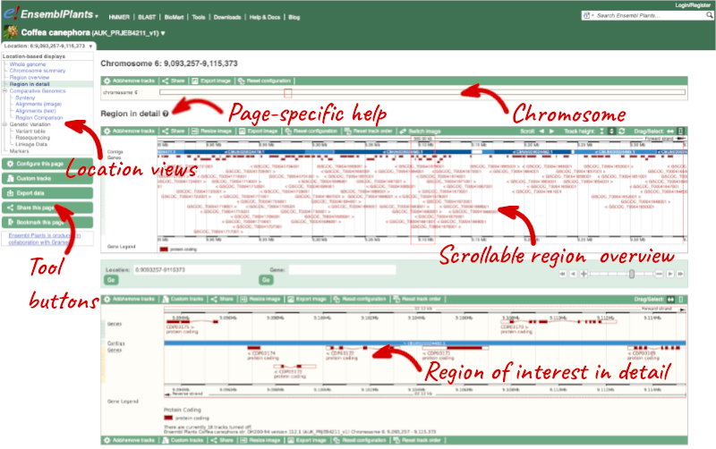
Click on the  button to view page-specific help. The help pages provide text, labelled images and, in some cases, help videos to describe what you can see on the page and how to interact with it.
The Region in detail page is made up of three images, let’s look at each one in detail.
- The first image shows the chromosome:
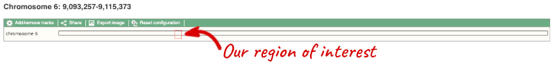
The region we’re looking at is highlighted on the chromosome.
- The second image shows a 1Mb region around our selected region. This is always 1Mb in human, but the fixed size of this view varies between species. This view allows you to scroll back and forth along the chromosome.
You can also drag out and jump to or mark a region.
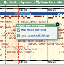
Click on the X to close the pop-up menu.
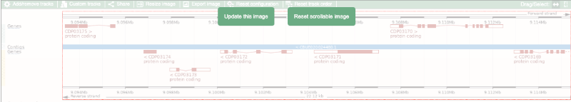
Click on the Drag/Select button  to change the action of your mouse click. Now you can scroll along the chromosome by clicking and dragging within the image. As you do this you’ll see the image below grey out and two blue buttons appear. Clicking on Update this image would jump the lower image to the region central to the scrollable image. We want to go back to where we started, so we’ll click on Reset scrollable image.
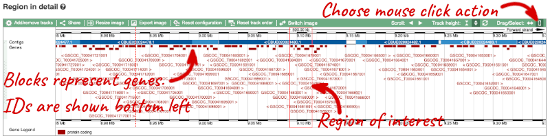
- The third image is a detailed, configurable view of the region.
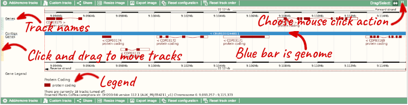
Here you can see various tracks, which is what we call a data type that you can plot against the genome. Some tracks, such as the transcripts, can be on the forward or reverse strand. Forward stranded features are shown above the blue contig track that runs across the middle of the image, with reverse stranded features below the contig. Other tracks, such as variants, regulatory features or conserved regions, refer to both strands of the genome, and these are shown by default at the very top or very bottom of the view.
You can use click and drag to either navigate around the region or highlight regions of interest, Click on the Drag/Select option at the top or bottom right to switch mouse action. On Drag, you can click and drag left or right to move along the genome, the page will reload when you drop the mouse button. On Select you can drag out a box to highlight or zoom in on a region of interest.
With the tool set to Select, drag out a box around an exon and choose Mark region.
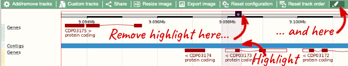
The highlight will remain in place if you zoom in and out or move around the region. This allows you to keep track of regions or features of interest.
We can edit what we see on this page by clicking on the blue Configure this page menu at the left.

This will open a menu that allows you to change the image.
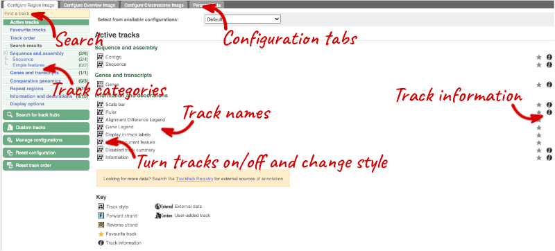
There are thousands of possible tracks that you can add. When you launch the view, you will see all the tracks that are currently turned on with their names on the left and an info icon on the right, which you can click on to expand the description of the track. Turn them on or off, or change the track style by clicking on the box next to the name. More details about the different track styles are in this FAQ.
You can find more tracks to add by either exploring the categories on the left, or using the Find a track option at the top left. Type in a word or phrase to find tracks with it in the track name or description.
Let’s add a track to this image. Add:
- All Repeats
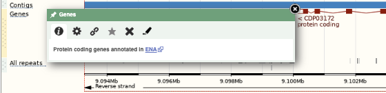
Now click on the tick in the top left hand to save and close the menu. Alternatively, click anywhere outside of the menu. We can now see the tracks in the image.
If the track is not giving you can information you need, you can easily change the way the tracks appear by hovering over the track name then the cog wheel to open a menu. To make it easier to compare information between tracks, such as spotting overlaps, you can move tracks around by clicking and dragging on the bar to the left of the track name.
Now that you’ve got the view how you want it, you might like to show something you’ve found to a colleague or collaborator. Click on the Share this page button to generate a link. Email the link to someone else, so that they can see the same view as you, including all the tracks you’ve added. These links contain the Ensembl release number, so if a new release or even assembly comes out, your link will just take you to the archive site for the release it was made on.

To return this to the default view, go to Configure this page and select Reset configuration at the bottom of the menu.
Exploring a genomic region in coffee
Go to Ensembl Plants.
-
Go to the region from 23,704,000 to 23,766,000 bp on coffee chromosome 1.
-
Zoom in on the GSCOC_T00030044001 gene with transcript ID CDP09644.
-
Configure this page to turn on the Repeats (Repbase) track in this view. What tool was used to annotate the repeats according to the track information? How many repeats can you see within the GSCOC_T00030044001 gene? Do any overlap exons?
-
Create a Share link for this display. Email it to your neighbour. Open the link they sent you and compare. If there are differences, can you work out why?
-
Export the genomic sequence of the region you are looking at in FASTA format.
-
Turn off all tracks you added to the Region in detail page.
-
Go to the Ensembl Plants homepage, select Coffea canephora from the Species drop-down list and type
1:23704000-23766000in the text box. Click Go. -
Draw with your mouse a box encompassing the GSCOC_T00030044001 transcript (with ID CDP09644). Click on Jump to region in the pop-up menu.
- Click Configure this page in the side menu (or on the cog wheel icon in the top left hand side of the bottom image). Go into Repeat regions in the left-hand menu then select Repeats (Repbase). Click on the (i) button to find out more information.
Repeats identified by RepeatMasker, using the Repbase library of repeat profiles.
Save and close the new configuration by clicking on ✓ (or anywhere outside the pop-up window). There are no repeats from Repbase overlapping GSCOC_T00030044001. -
Click Share this page in the side menu. Copy the URL. Get your neighbour’s email address and compose an email to them, paste the link in and send the message. When you receive the link from them, open the email and click on your link. You should be able to view the page with the new configuration and data tracks they have added to in the Location tab. You might see differences where they specified a slightly different region to you, or where they have added different tracks.
-
Click Export data in the side menu. Leave the default parameters as they are (FASTA sequence should already be selected). Click Next>. Click on Text. Note that the sequence has a header that provides information about the genome assembly, the chromosome, the start and end coordinates and the strand. For example:
>1 dna:chromosome chromosome:AUK_PRJEB4211_v1:1:23755890:23764847:1 - Click Configure this page in the side menu. Click Reset configuration. Click ✓.
Genes and Transcripts
You can find out lots of information about Ensembl genes and transcripts using the browser. If you’re already looking at a region view, you can click on any transcript and a pop-up menu will appear, allowing you to jump directly to that gene or transcript.
Alternatively, you can find a gene by searching for it. You can search for gene names or identifiers, and also phenotypes or functions that might be associated with the genes.
We’re going to look at the Coffea canephora GSCOC_T00022371001 gene. From plants.ensembl.org, type GSCOC_T00022371001 into the search bar and click the Go button.
The gene tab
Click on GSCOC_T00022371001 from the search hits. The Gene tab should open:
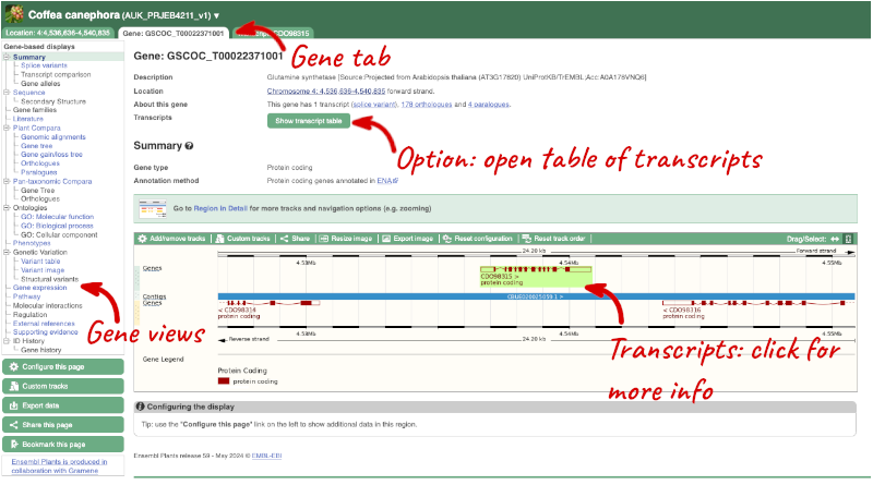
This page summarises the gene, including its location, name and equivalents in other databases. At the bottom of the page, a graphic shows a region view with the transcripts. We can see exons shown as blocks with introns as lines linking them together. Coding exons are filled, whereas non-coding exons are empty. We can also see the overlapping and neighbouring genes and other genomic features.
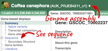
There are different tabs for different types of features, such as genes, transcripts or variants. These appear side-by-side across the blue bar, allowing you to jump back and forth between features of interest. Each tab has its own navigation column down the left hand side of the page, listing all the things you can see for this feature.
Let’s walk through this menu for the gene tab. How can we view the genomic sequence? Click Sequence at the left of the page.
The sequence is shown in FASTA format. The FASTA header contains the genome assembly, chromosome, coordinates and strand (1 or -1) – this gene is on the positive strand.
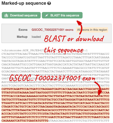
Exons are highlighted within the genomic sequence, both exons of our gene of interest and any neighbouring or overlapping gene. By default, 600 bases are shown up and downstream of the gene. We can make changes to how this sequence appears with the blue Configure this page button found at the left. This allows us to change the flanking regions, add line numbering and more. Click on it now.
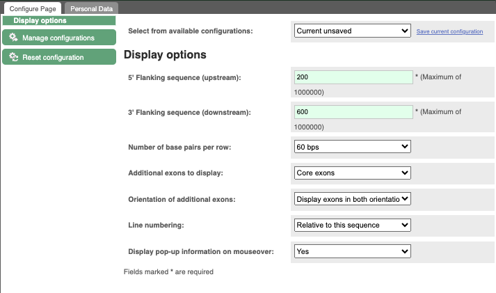
Once you have selected changes (in this example, Line numbering) click at the top right.

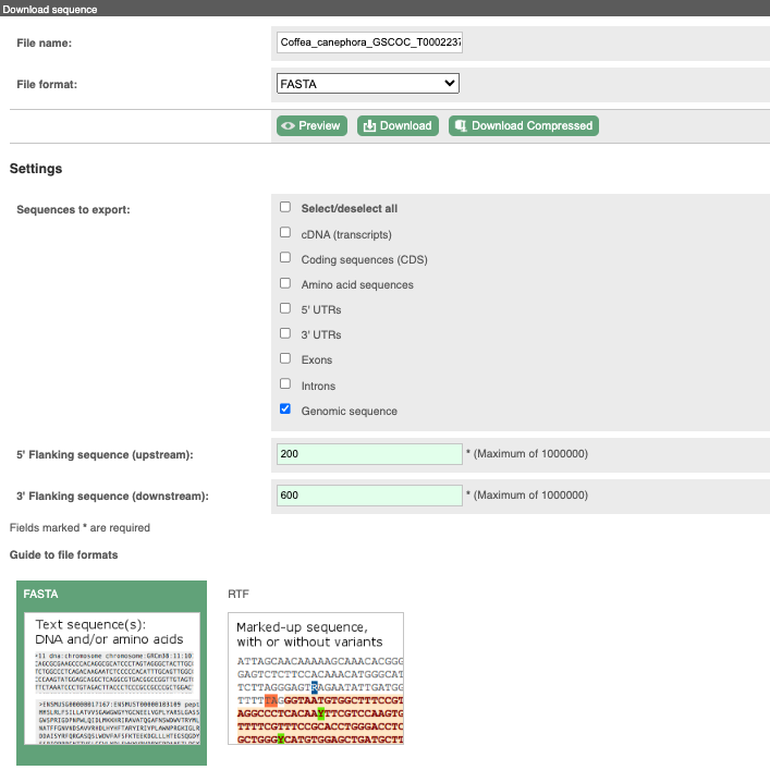
You can download this sequence by clicking in the Download sequence button above the sequence:
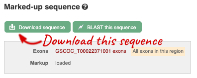
This will open a dialogue box that allows you to pick between plain FASTA sequence, or sequence in RTF, which includes all the coloured annotations and can be opened in a word processor. If you want run a sequence analysis tool, download as FASTA sequence, whereas if you want to analyse the sequence visually, RTF is best for this. This button is available for all sequence views.
To find out what the protein does, have a look at GO terms from the Gene Ontology consortium. There are three pages of GO terms, representing the three divisions in GO: Biological process (what the protein does), Cellular component (where the protein is) and Molecular function (how it does it). Click on GO: Biological process to see an example of the GO pages.
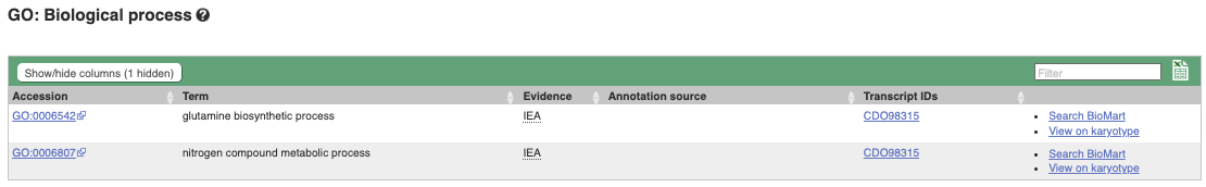
Here you can see the functions that have been associated with the gene. There are three-letter codes that indicate how the association was made, as well as links to the specific transcript they are linked to.
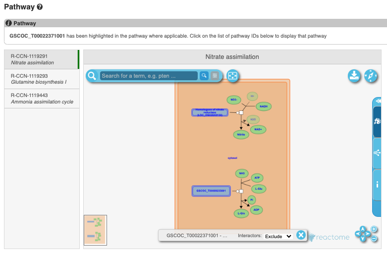
To find the biochemical pathways that this gene is involved in, from Reactome, click on Pathway in the left-hand menu
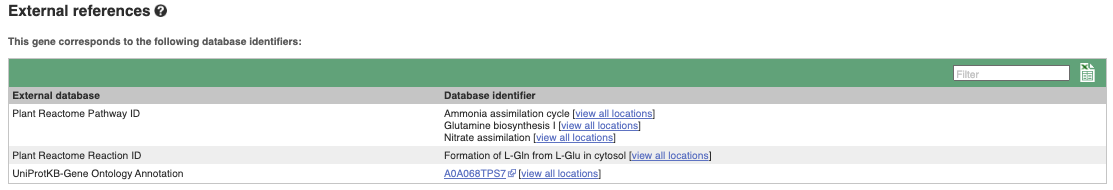
We also have links out to other databases which have information about our genes and may focus on other topics that we don’t cover, like Expression Atlas or UniProtKB. Go up the left-hand menu to External references:
Demo: The transcript tab
We’re now going to explore the different transcripts of GSCOC_T00022371001. Click on Show transcript table at the top.
![]()
![]()
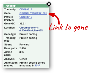
Here we can see that there is only one transcript of GSCOC_T00022371001 with its identifier, length and biotype. Click on the ID of the Ensembl Canonical transcript, CDO98315.
You are now in the Transcript tab for CDO98315. We can still see the gene tab so we can easily jump back. The left hand navigation column provides several options for the transcript CDO98315 - many of these are similar to the options you see in the gene tab, but not all of them. If you can’t find the thing you’re looking for, often the solution is to switch tabs.
Click on the Exons link. This page is useful for designing RT-PCR primers because you can see the sequences of the different exons and their lengths.
![]()
You may want to change the display (for example, to show more flanking sequence, or to show full introns). In order to do so click on Configure this page and change the display options accordingly.
Now click on the cDNA link to see the spliced transcript sequence with the amino acid sequence. This page is useful for mapping between the RNA and protein sequences, particularly genetic variants.
![]()
UnTranslated Regions (UTRs) are highlighted in dark yellow, codons are highlighted in light yellow, and exon sequence is shown in black or blue letters to show exon divides. Sequence variants are represented by highlighted nucleotides and clickable IUPAC codes are above the sequence.
Next, follow the General identifiers link at the left. Just like the External References page in the gene tab, this page shows links out to other databases such as RefSeq, UniProtKB, PDBe and others, this time linked to the transcript or protein product, rather than the gene.
![]()
If you’re interested in protein domains, you could click on Protein summary to view domains from Pfam, PROSITE, Superfamily, InterPro, and more. These are all plotted against the transcript sequence, with the exons shown in alternating shades of purple at the top of the page. Alternatively, you can go to Domains & features to see a table of the same information.
![]()
![]()
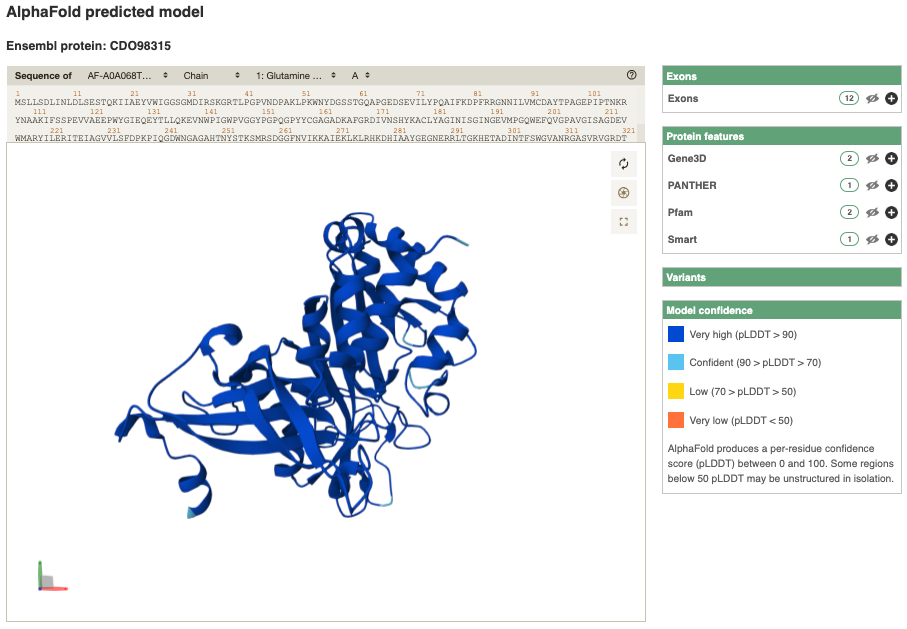
You can also view the AlphaFold predicted 3D structure of the protein. Click on AlphaFold predicted model in the left-hand menu.
Exploring the FUS3 gene in Coffea canephora (Robusta coffee)
The FUS3 gene is a known master regulator of somatic embryogenesis, an important factor in stable genetic transformation and successful plant regeneration of coffee trees expressing the Bacillus thuringiensis (Bt) toxin Cry10Aa to induce Coffee Berry Borer (CBB) resistance.
-
Find the Coffea canephora FUS3 gene on Ensembl Plants. On which chromosome and which strand of the genome is this gene located?
-
Where in the cell is the FUS3 protein located?
-
What is the source of the assigned gene description?
-
How long is its transcript (in bp)? How long is the protein it encodes? How many exons does it have? Are any of the exons completely or partially untranslated?
- Go to the Ensembl Plants homepage (http://plants.ensembl.org/). Select C. canephora from the species list and type
FUS3in the search box. Click Go and click on the gene ID GSCOC_T00019208001. You can find the strand orientation and the location under Summary in the Gene tab.The C. canephora FUS3 gene is located on chromosome 7 on the forward strand.
- Click on GO: Cellular component in the left-hand panel.
The protein is located in the nucleus.
- Click on Summary in the side menu.
The gene description is Projected from Arabidopsis thaliana (AT3G26790) by UniProtKB/Swiss-Prot;Acc:Q9LW31.
- Click on Show transcript table.
The transcript is 1038 bp and the length of the encoded protein is 279 amino acids.
Click on the transcript ID CDP16731 in the transcript table. You can find the number of exons in under in the summary information at the top of the page.
It has 7 exons.
Click on Sequence: Exons in the left-hand panel.
The last exon is partially untranslated (sequence shown in orange). This can also been seen from the fact that in the transcript diagrams on the Gene Summary and Transcript Summary pages the boxes representing the last exon is partially unfilled.
Exploring a fungal gene in Rosellinia necatrix
Rosellinia necatrix is is a fungal plant pathogen infecting several hosts including coffee, apples, apricots, avocados, cassava, strawberries, pears, hop, citruses and Narcissus, causing white root rot. A study by A. Zumaquero et al in 2019 (doi: 10.1186/s12864-019-6387-5) revealed SAMD00023353_4000440 as a gene potentially involved in pathogenesis.
Start in Ensembl Fungi and select the Rosellinia necatrix str. W97 (GCA_001445595) genome.
-
What GO: molecular function terms are associated with the SAMD00023353_4000440 gene?
-
Go to the transcript tab for the only transcript, GAP89412. How long is the transcript?
-
What domains can be found in the protein product of this transcript? How many different domain prediction methods agree with each of these domains?
- From the Ensembl Fungi homepage, select Rosellinia necatrix str. W97 (GCA_001445595) by selecting the species from the table of species. Type
SAMD00023353_4000440and click on the gene ID SAMD00023353_4000440. Click on GO: molecular function in the left-hand panel.There is one term listed: GO:0004190, aspartic-type endopeptidase activity.
- Click on the transcript named GAP89412 or on the Transcript tab.
GAP89412 is 1413 bp in length.
- Click on either Protein Summary or Domains & features in the left hand menu to see the predicted domains and motifs graphically or as a table respectively. You can also click on AlphaFold predicted model to view the AlphaFold predicted 3D structure of the protein.
Variation
Exploring variants in Arabidopsis thaliana
Visualising variants in the Sequence view
In any of the sequence views shown in the Gene and Transcript tabs, you can view variants on the sequence. You can do this by clicking on Configure this page from any of these views.
Let’s take a look at the Gene sequence view for PAD4 in Arabidopsis thaliana. Search for PAD4 and go to the Sequence view.
If you can’t see variants marked on this view, click on Configure this page and select Show variants: Yes and show links.
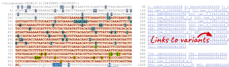
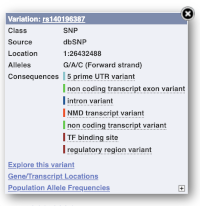
Find out more about a variant by clicking on it.
You can add variants to all other sequence views in the same way.
You can go to the Variation tab by clicking on the variant ID. For now, we’ll explore more ways of finding variants.
Viewing variants within a gene in the tabular form
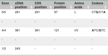
To view all the sequence variants in table form, click the Variant table link at the left of the gene tab.
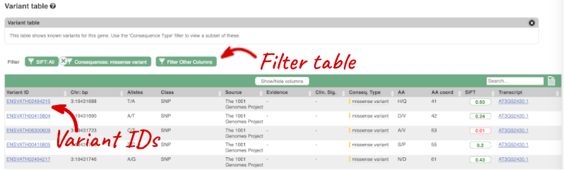
You can filter the table to only show the variants you’re interested in. For example, click on Consequences: All, then select the variant consequences you’re interested in. For display purposes, the table above has already been filtered to only show missense variants.
You can also filter by the different pathogenicity scores and MAF, or click on Filter other columns for filtering by other columns such as Evidence or Class.
The table contains lots of information about the variants. You can click on the IDs here to go to the Variation tab too.
Visualising variants in the Region in Detail view
Let’s have a look at variants in the Location tab. Click on the Location tab in the top bar.
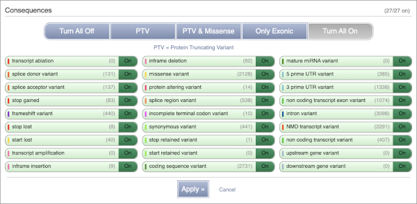
Configure this page and open Variation from the left-hand menu.
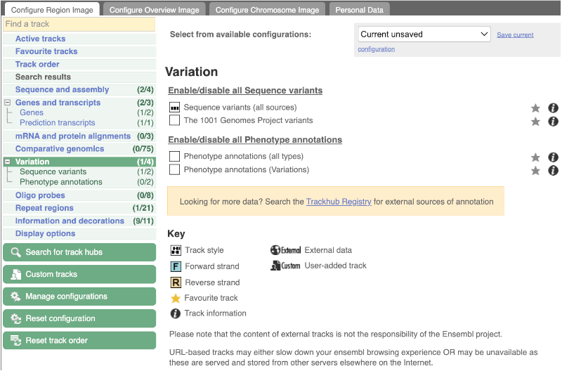
There are various options for turning on variants. You can turn on variants by source or presence of a phenotype. You can also turn on genotyping chips.
Turn on Sequence Variants (all sources) in Normal format.
Exploring a specific variant
Let’s have a look at a specific variant. If we zoomed in we could see the variant tmp_319431818_G_C in this region, however it’s easier to find if we put _tmp_3_19431818_G_C into the search box. Click through to open the Variation tab for Arabidopsis thaliana.
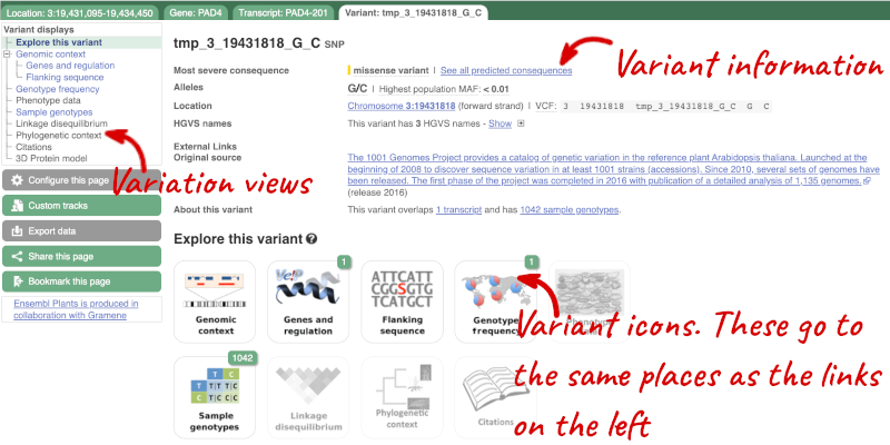
The icons show you what information is available for this variant. Click on Genes and regulation, or follow the link on the left.
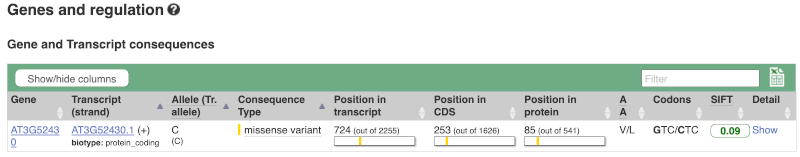
This page illustrates the genes the variant falls within and the consequences on those genes, including pathogenicity predictors.
Let’s look at population genetics. Click on Population genetics in the left-hand menu.
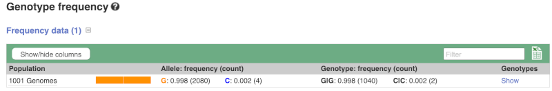
The population allele frequencies are shown by study. Where genotype frequencies are available, these are shown in the tables.
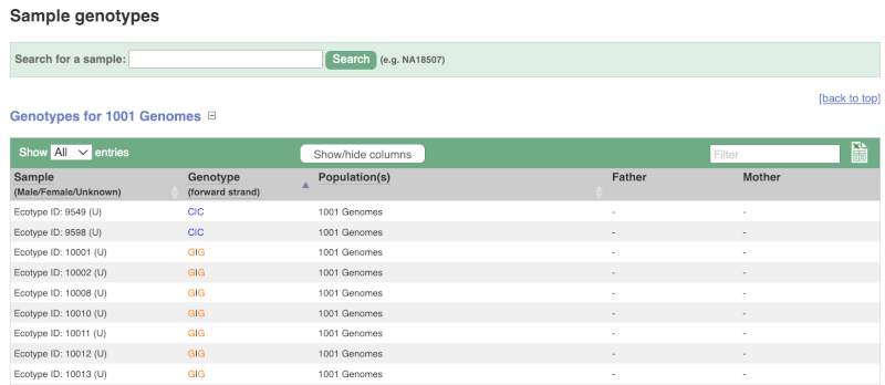
We can see which strains these genotypes were observed in by going to Sample Genotypes.
Exploring a SNP in Arabidopsis
The Arabidopsis thaliana ATCDSP32 protein is a chloroplastic drought-induced stress protein proposed to participate in a process called cell redox homeostasis. Go to Ensembl Plants and answer the following questions:
-
How many variants have been identified in the gene that can cause a change in the protein sequence (i.e. missense variant)?
-
What is the ID of the variant that changes the amino acid residue 60 from Alanine to Threonine (hint: refer to an amino acid codon table)? What is the location of this SNP in the A. thaliana genome? What are its possible alleles?
-
Download the flanking sequence of this SNP in RTF (Rich Text Format). Can you change how much flanking sequence is displayed on the browser?
-
Does this SNP cause a change at the amino acid level for other genes or transcripts?
- Click on Arabidospsis thaliana on the Ensembl Plants homepage. Search for ATCDSP32 on the species page and in the search results, click on the Gene ID AT1G76080. In the left-hand side menu of the Gene tab, click on Variant table. Click on Consequences: All then select only missense variant.
The missense variant button indicates that there are 18 of these. Alternatively, you can count the number of variants in your filtered list.
- An amino acid codon table can be found on Wikipedia. Sort the AA coord column by clicking on the header and scroll down to find a variant at residue 60. The ID of this variant is ENSVATH05153232.
The variant is located at position 28549171 on chromosome 1. The two possible alleles at this locus are C (reference) and T (alternative).
- Click on the link ENSVATH05153232, then click on Flanking sequence in the left-hand side menu. Now click on Download sequence and select File format > Rich Text Format (RTF).
If you want to change how much flanking sequence is displayed on the browser, go back to the Flanking sequence page, click on the Configuration button and change the length of the sequence. The default settings is 400 bp.
- Click on Genes and regulation in the left-hand side menu.
This SNP does not cause a change at the amino acid level for any other genes or transcripts in A. thaliana.
Variation data in tomato
-
Go to Ensembl Plants and find the Solyc02g084570.3 gene in Solanum lycopersicum (tomato) and go to its Location tab. Can you see the variation track?
-
Zoom in around the last exon of this gene. What are the different types of variants seen in that region? Are any splice region variants mapped in the region? If so, what is/are the coordinate(s)?
- Select Solanum lycopersicum from the Species search drop-down menu and search for
Solyc02g084570.3. In the results page, you can click on the coordinates 2:48284598-48288482 to go straight to the Location tab. Scroll down to the Region in detail view. The variation track is shown at the bottom of the view.If you don’t see the Variation - All sources track, click Configure this page on the left-hand panel, search for the track in the pop-up menu and enable the track by clicking on the square next to the track name. Close the pop-up window and wait for the track to load.
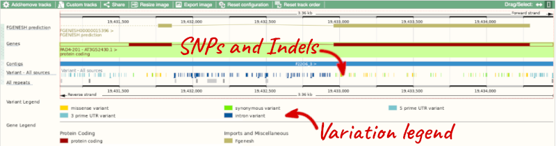
- Zoom in around the last exon of this gene by drawing a box in the respective region (you can change your mouse action by clicking the Drag/Select icons at the top right-hand corner of the view). Note the gene is on the reverse strand (this is signified by the < sign next to the transcript name, and it is located below the Contigs track), so the last exon will be on the left hand side of that image. The variation legend is shown at the bottom of the page, telling you what the colours mean.
The types of variants seen in that region are 3’ UTR, missense, synonymous and splice region variants.
Splice region variants are shown in orange. Click on the variants to get additional information on that variant including location. You can zoom into the region if the variant block is too small to click.
The variants are found at 2:48285642 and 2:48285640-48285641. Note that the two variants overlap: one is a SNP and the other is an indel. SNPs are tagged with ambiguity codes (zoom into the region if you cannot see this). You can find a useful IUPAC ambiguity code guid on the bioinformatics.org website. Single-letter ambiguity codes are given when two or more possible nucleotides may be represented at a single base locus.
VEP
Demonstration of the VEP web interface
Input
We have identified three variants on coffee chromosome 4:
T -> C at 25759812
G -> A at 25685623
T -> G at 25863697
We will use the Ensembl VEP to determine which genes are affected by my variants?
Click on Tools in the top green bar from any Ensembl Plants page, then Variant Effect Predictor to open the input form:
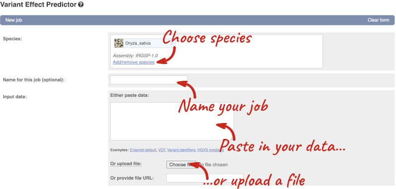
Click on Add/remove species and search for Triticum aestivum to choose it.
The data is in VCF:
chromosome coordinate id reference alternative
Put the following into the Paste data box:
4 25759812 var1 T C
4 25685623 var2 G A
4 25863697 var3 T G
The VEP will automatically detect that the data is in VCF.
Additional configurations
There are further options that you can choose for your output. These are categorised as Identifiers, Variants and frequency data, Additional annotations, Predictions, Filtering options and Advanced options. Let’s open all the menus and take a look.
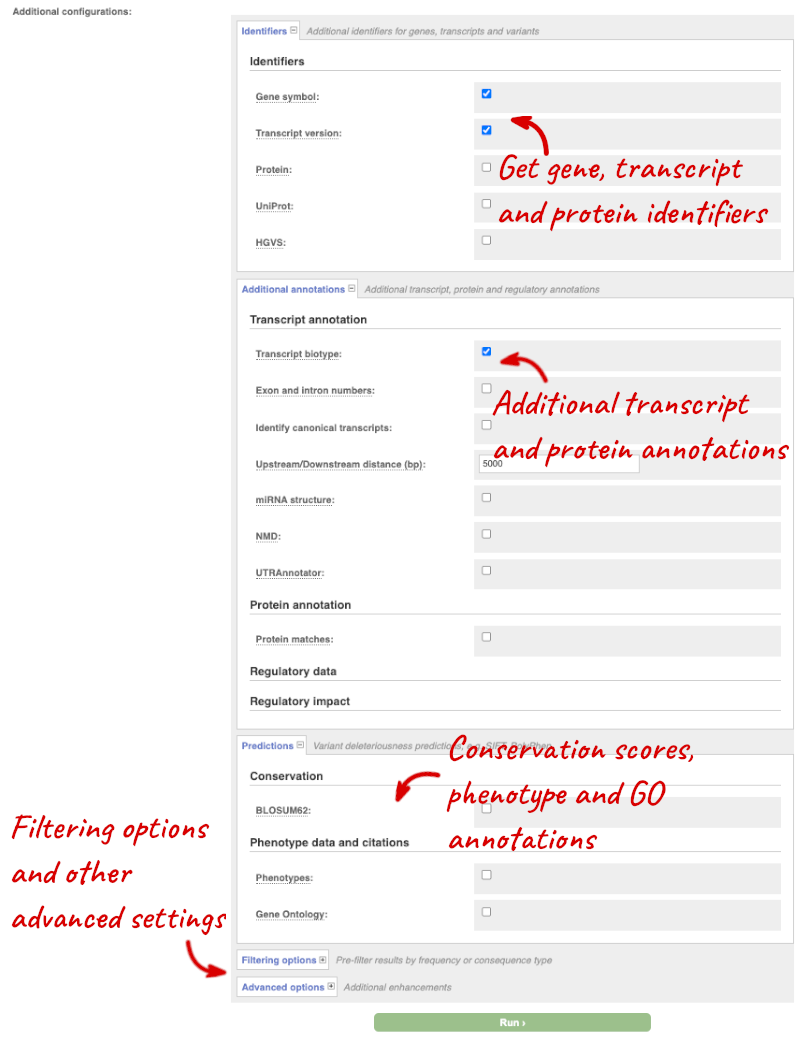
Hover over the options to see definitions.
When you’ve selected everything you need, scroll right to the bottom and click Run.

The display will show you the status of your job. It will say Queued, then automatically switch to Done when the job is done, you do not need to refresh the page. You can edit or discard your job at this time. If you have submitted multiple jobs, they will all appear here.
Click View results once your job is done.
Results
In your results you will see a graphical summary of your data, as well as a table of your results.
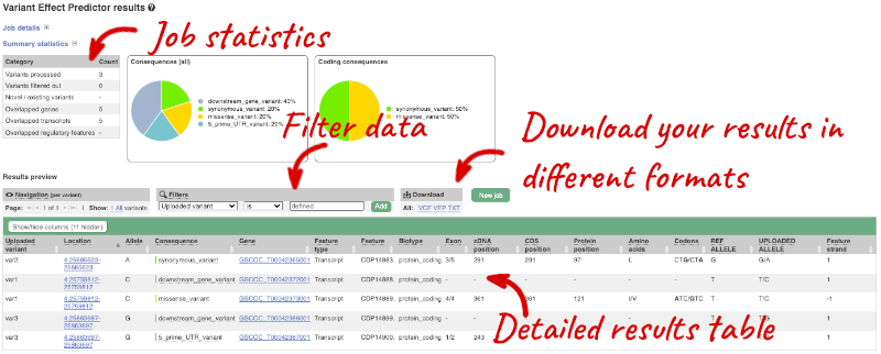
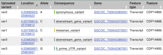
The results table is enormous and detailed, so we’re going to go through the it by section. The first column is Uploaded variant. If your input data contains IDs, like ours does, the ID is listed here. If your input data is only loci, this column will contain the locus and alleles of the variant. You’ll notice that the variants are not neccessarily in the order they were in in your input. You’ll also see that there are multiple lines in the table for each variant, with each line representing one transcript or other feature the variant affects.
You can mouse over any column name to get a definition of what is shown.
The next few columns give the information about the feature the variant affects, including the consequence. Where the feature is a transcript, you will see the gene symbol and stable ID and the transcript stable ID and biotype. The IDs are links to take you to the gene or transcript homepage.
This is followed by details on the effects on transcripts, including the position of the variant in terms of the exon number, cDNA, CDS and protein, as well as the amino acid and codon change.
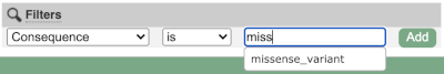
Above the table is the Filter option, which allows you to filter by any column in the table. You can select a column from the drop-down, then a logic option from the next drop-down, then type in your filter to the following box. We’ll try a filter of Consequence, followed by is then missense_variant, which will give us only variants that change the amino acid sequence of the protein. You’ll notice that as you type missense_variant, the VEP will make suggestions for an autocomplete.
You can export your VEP results in various formats, including VCF. When you export as VCF, you’ll get all the VEP annotation listed under CSQ in the INFO column. After filtering your data, you’ll see that you have the option to export only the filtered data. You can also drop all the genes you’ve found into the Gene BioMart, or all the known variants into the Variation BioMart to export further information about them.
Web VEP analysis of variants in Coffea canephora (coffee)
You have done whole-genome sequencing and variant-calling experiments for Coffea canephora. You have a VCF file with a small subset of variants from this experiment. Analyse the variants in this file with the VEP tool in Ensembl Plants and determine the following:
1 35246062 var1 C A
1 35246078 var2 G C
1 35246154 var3 T A
-
How many genes and transcripts are affected by variants in this file?
-
Filter the table to find variants with high impact. How many variants have high impact and what consequence predictions do they refer to? Why do you think missense variants are not classified as high impact?
-
Can you export all the results to a VCF file? Compare it to the input VCF file to see what information the VEP adds.
Go to any Ensembl Plants page and click on Tools in the navigation bar at the top of the page. Click on Variant Effect Predictor and change your species to Triticum aestivum by clicking on Change species.
Enter a descriptive name for your VEP job. Paste the variants in VCF format into the text box. Click Run at the bottom of the page. When your job is done, click View reesults.
-
Only 1 gene is affected by variants in this file. The gene has 1 transcript which is affected by the variants.
- Use the filters to view only variants with HIGH impact (you may need to add the column under Show/hide columns at the top of the table if you cannot find it). The filters are found above the detailed results table in the middle. Select Impact and is from the drop-down menus. Then type
HIGHinto the box; this will autocomplete. Click Add.There are 2 variants with high impact (var1 ands var3). One is a start lost (although also a start retained variant), the other is a splice donor variant. Missense variants are not classified as high impact, because they do not always have significant impacts on protein functions. Usually the protein is still produced. In contrast, start/stop altering variants affect the protein length, and therefore likely affect the protein function.
- At the top right of the table there is an option to download data. Click on VCF for the All option. Open the VCF file you have downloaded in a text editor. You can see that VEP adds annotation in the INFO column of the VCF file.
Comparative genomics
Demo: gene trees and homology predictions
Plants Compara
Gene trees
Let’s look at the homologues of Coffea canephora (coffee) GSCOC_T00022371001. Open Ensembl Plants, search for the gene and go to the Gene tab.
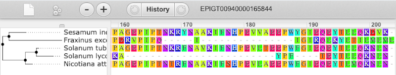
Click on Plant compara: Gene tree, which will display the current gene in the context of a phylogenetic tree used to determine orthologues and paralogues.
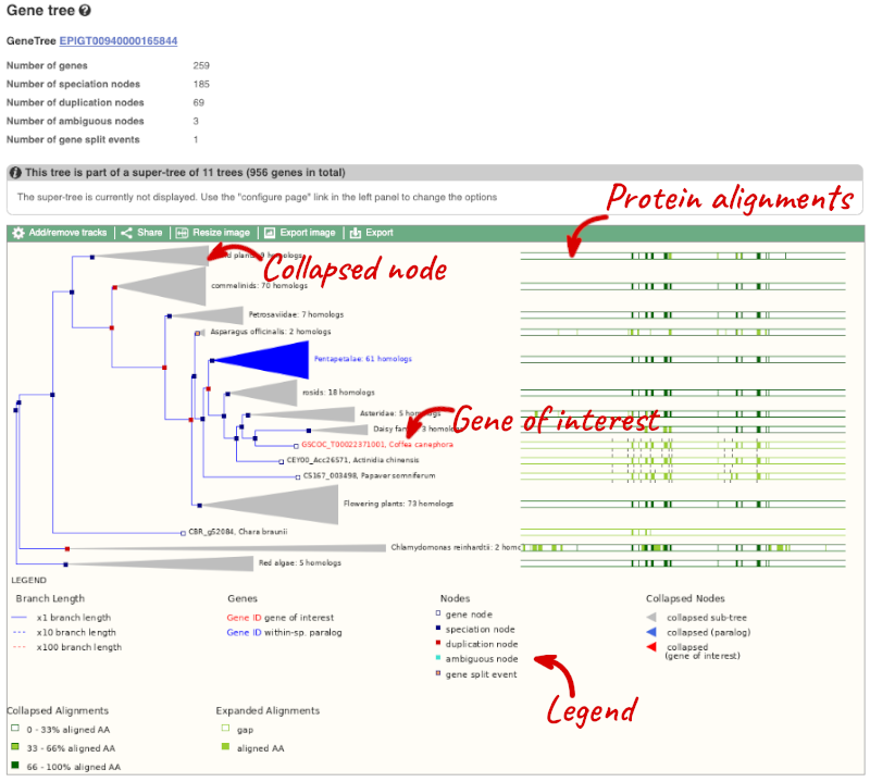
Funnels indicate collapsed nodes. We can expand them by clicking on the node and selecting Expand this sub-tree from the pop-up menu.
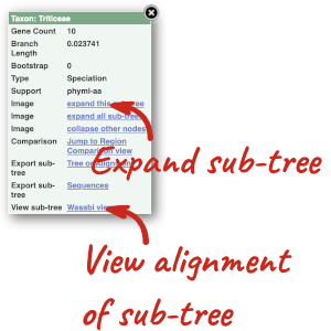
We can also see the protein alignment of the sub-tree by clicking on Wasabi viewer, which will open a pop-up:
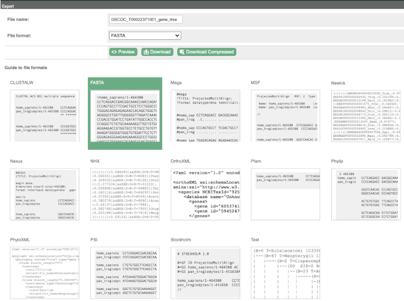
You can download the tree in a variety of formats. Click on the download icon ![]() in the bar at the top of the image to get a pop-up where you can choose your format.
in the bar at the top of the image to get a pop-up where you can choose your format.
Homologues
We can look at homologues in the Orthologues and Paralogues pages, which can be accessed from the left-hand menu. If there are no orthologues or paralogues, then the name will be greyed out. Click on Plant compara: Orthologues to see the orthologues available in plants.
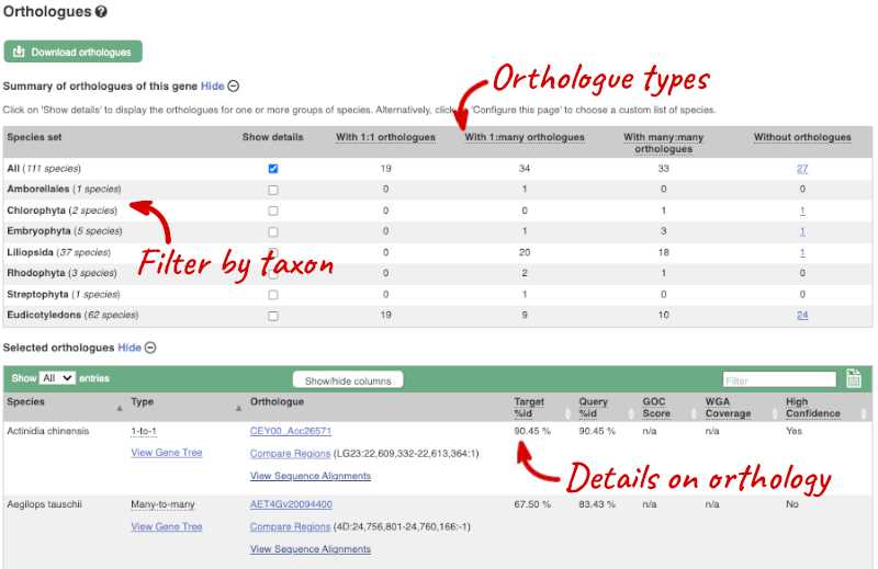
Choose to see only Eudicotyledons orthologues by selecting the box. The table below will now only show details of Eudicotyledons orthologues. Let’s look at Arabidopsis thaliana.
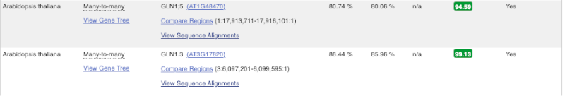
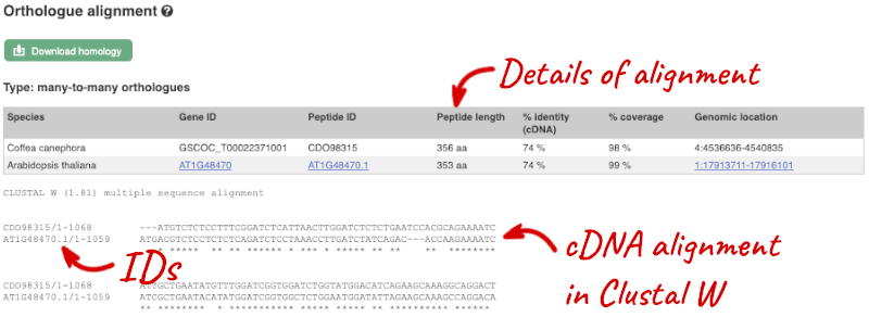
Here we can see there is a many-to-many relationship between the coffee and A. thaliana orthologues. Links from the orthologue allow you to go to alignments of the orthologous proteins and cDNAs. Click on View Sequence Alignments then View cDNA Alignment for the first A. thaliana orthologue.
Demo: Whole-genome alignments
Alignments in the Region in Detail view
Let’s look at some of the comparative genomics views in the Location tab. Go to the region 4:4:4640000-4680000 in Coffea canephora (coffee). We can look at individual species comparative genomics tracks in this view by clicking on Configure this page.
Select Comparative genomics from the left-hand menu to choose alignments between closely related species. Turn on the alignments for Arabidopsis thaliana, Oryza sativa japonica Group (rice) and Solanum lycopersicum (tomato).
Sequence alignments
We can also look at the alignment between species or groups of species as text. Click on Comparative Genomics: Alignments (text) in the left-hand menu.
Click on Select an alignment to open the alignment menu. Select A. thaliana from the alignments list then click Go.
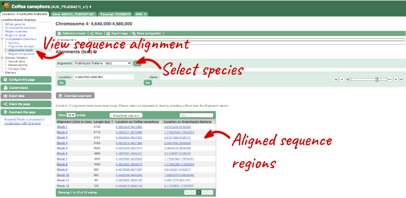
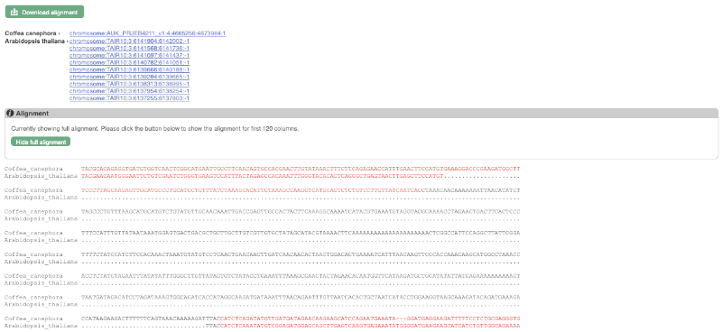
In this case there are 12 blocks aligned of different lengths. Click on Block 1.
You will see a list of the regions aligned, followed by the sequence alignment. Click on Display full alignment. Exons are shown in red (you may need to scroll down the page to see the first exon).
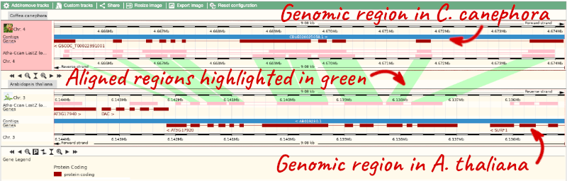
Region comparison
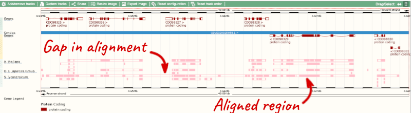
To compare with both contigs visually, go to Comparative Genomics: Region Comparison.
To add species to this view, click on the green Select species or regions button. Choose A. thaliana again then close the menu.
Synteny
We can view large-scale syntenic regions from our chromosome of interest. Click on Comparative Genomics: Synteny in the left-hand menu and select S. lycopersicum* from the **Change species drop-down in the right-hand side.
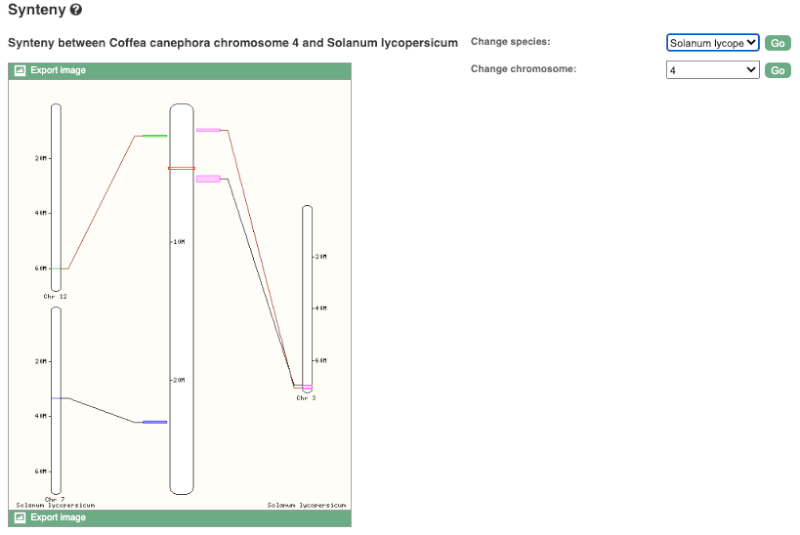
Black linking lines indicate sequences are oriented in the same directed, red linking lines indicate the sequences are inverted.
Finding orthologous genes for disease resistance gene in Coffea canephora (coffee)
Resistance to the leaf rust delivered by SH3 factor(s) is well-grounded as specially durable. in 2023, Paula Cristina da Silva Angelo et al (https://doi.org/10.1016/j.pmpp.2023.102111) reported that the Arabidopsis thaliana gene AT1G50180 is an important gene in the SH3 locus conferring diseae resistance.
Search Ensembl Plants for the gene AT1G50180 in Arabidopsis thaliana.
-
From the gene tab, go to the Arabidopsis thaliana AT1G50180 gene Orthologues page under Plant Compara.
-
Reduce the orthologues table to look only at Coffea canephora (coffee) orthologues. How many results can you see?
-
Download the cDNA alignment in ClustalW format for the alignment between the Arabidopsis thaliana AT1G50180 gene and the Coffea canephora GSCOC_T00030728001 gene.
Go to Ensembl Plants. Select Arabidopsis thaliana from the drop-down box and type in AT1G50180. Click Go and click on the gene ID AT1G50180.
-
Go to Plant Compara: Orthologues on the left-hand panel.
- Filter for Coffea canephora using the filter option in the top right hand corner of the table.
Coffee has 25 many-to-many orthologues.
- Click on View Sequence Alignments then cDNA (found in the 3rd column below the gene identifier) for the GSCOC_T00030728001 gene. This takes us to the Orthologue Alignment page.
Click on Download Homology to download the alignment in ClustalW format
BioMart
Demo: BioMart
Follow these instructions to guide you through BioMart to answer the following query:
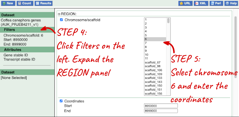
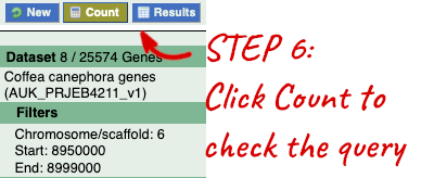
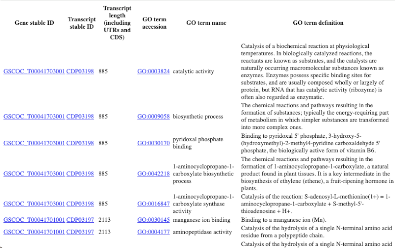
- What genes are found on chromosome 6, between 8950000 and 8999000 in coffee?
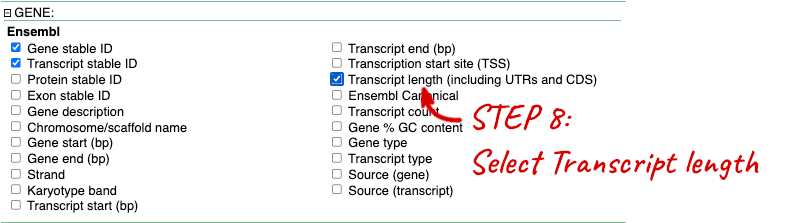
- What is the transcript length (UTR + CDS)?
- Are there associated functions from the GO (gene ontology) project that might help describe their function?
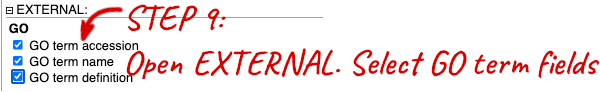
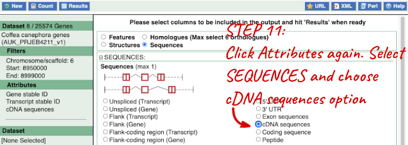
- What are their cDNA sequences?
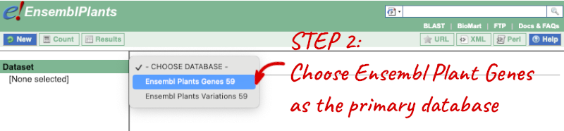
Step 1: Choose the database and dataset
Click on BioMart in the top header of any Ensembl Plants page to open BioMart
Step 2: Choose appropriate filters
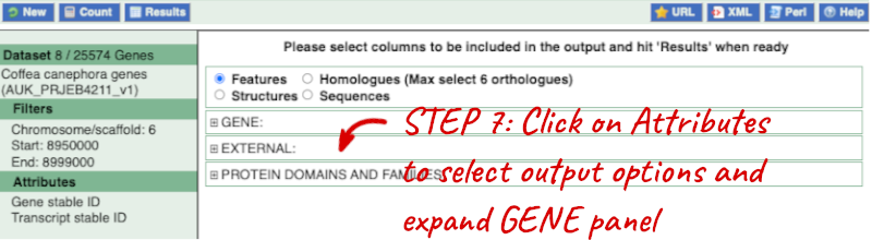
Step 3.1: Select attributes (features)
Step 4.1: Get the results
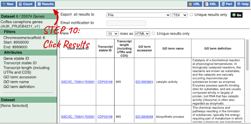
Why are there multiple rows for one gene ID? For example, look at the first few rows.
Step 3.2: Select attributes (sequences)
Step 4.2: Get the results
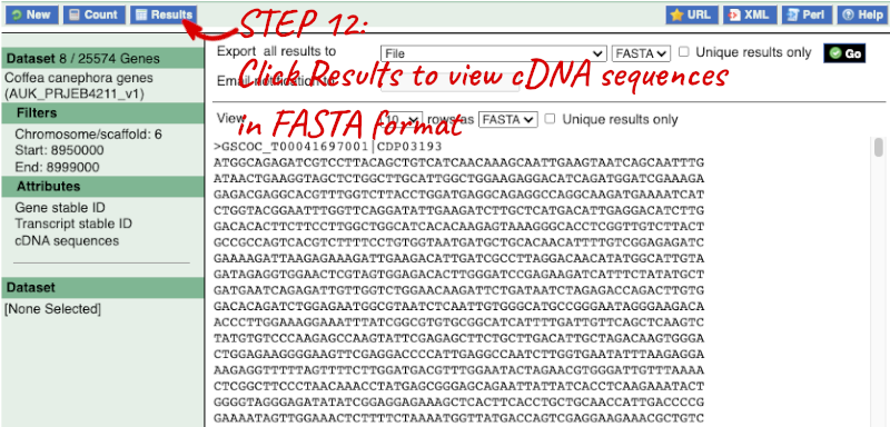
Note: you can use the Go button to export a file.
What did you learn about the coffee genes in this exercise?
Could you learn these things from the Ensembl browser? Would it take longer?
Finding genes by protein domain
Find Coffea canephora (coffee) proteins with Signalp cleavage sites located on chromosome 7.
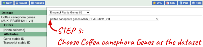
As with all BioMart queries you must select the dataset, set your filters (input) and define your attributes (desired output). For this exercise: Dataset: Ensembl Plant Genes in Coffea canephora Filters: Signalp cleavage sites on chromosome 7 Attributes: Gene stable ID and Transcript stable ID
Go to the Ensembl Plants homepage (https://plants.ensembl.org/index.html) and click on BioMart at the top of the page. Select Ensembl Plant Genes as your database and Coffea canephora genes as the dataset. Click on Filters on the left of the screen and expand REGION. Change the chromosome to 7. Now expand PROTEIN DOMAINS, also under filters, and select Limit to genes, choosing with With Cleavage site (Signalp) from the drop-down and then Only. Clicking on Count should reveal that you have filtered the dataset down to 192 genes.
Click on Attributes and expand GENE. Ensure Gene stable ID and Transcript stable ID are selected. Now click on Results. The first 10 results are displayed by default; Display all results by selecting ALL from the drop down menu.
The output will display the Ensembl gene IDs and Ensembl Transcript IDs of all proteins with a Signalp cleavage site on coffee chromosome 7. If you prefer, you can also export as an Excel sheet by using the Export all results to XLS option.
Exporting homologues with BioMart
Go to Ensembl Plants’s BioMart. For a list of Arabidopsis thaliana genes, export the coffee orthologues:
MLP28, MEE18, EP1, QRT3, MOT2, GC4, WYR
Do all of these genes have a homologue in coffee?
-
Go to BioMart (you can find a shortcut in the navigation bar at the top of any Ensembl Plants page) and click New. Choose the Ensembl Plant Genes database. Choose the Arabidopsis thaliana genes (TAIR10) dataset.
-
Click on Filters in the left panel. Expand the GENE. Enter the gene list in the Input external references ID list box. Select Gene Name from the input options dropdown list.
-
Click on Attributes in the left panel. Select the Homologues attributes at the top of the page. Expand the GENE section. Select Gene Name. Expand the ORTHOLOGUES [A-E] section. Select Coffea canephora gene stable ID.
-
Click Results. Select View: All rows as HTML.
All genes have a homologue in coffee.