Filter Events by Year
Exploring plant genes and genomes using the Ensembl REST API
Course Details
- Lead Trainer
- Ben Moore
- Associate Trainer
- Event Dates
- 2022-10-03 until 2023-10-05
- Location
- Virtual: Graphic Era Hill University (GEHU), Dehradun, India
- Description
- Work with the Ensembl Outreach team to get to grips with the Ensembl plants REST API.
- Survey
- Exploring plant genes and genomes using the Ensembl REST API Feedback Survey
Demos and exercises
Genes and transcripts
Demo: Exploring genes and transcripts in Ensembl Plants
You can find out lots of information about Ensembl genes and transcripts using the browser. If you’re already looking at a region view, you can click on any transcript and a pop-up menu will appear, allowing you to jump directly to that gene or transcript.
Alternatively, you can find a gene by searching for it. You can search for gene names or identifiers, and also phenotypes or functions that might be associated with the genes.
We’re going to look at the Arabidopsis thaliana PAI1 gene. From plants.ensembl.org, type PAI1 into the search bar and click the Go button.
The gene tab
Click on PAI1 from the search hits. The Gene tab should open:
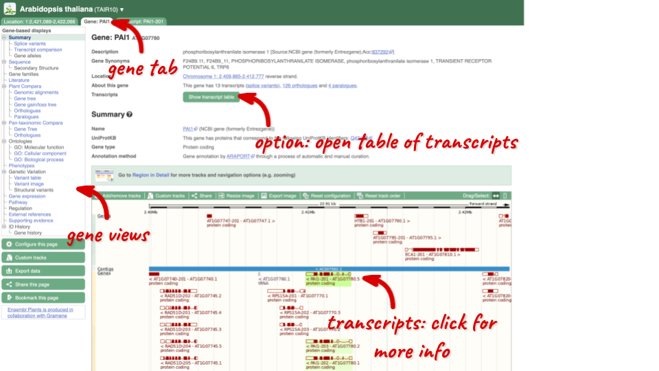
This page summarises the gene, including its location, name and equivalents in other databases. At the bottom of the page, a graphic shows a region view with the transcripts. We can see exons shown as blocks with introns as lines linking them together. Coding exons are filled, whereas non-coding exons are empty. We can also see the overlapping and neighbouring genes and other genomic features.
There are different tabs for different types of features, such as genes, transcripts or variants. These appear side-by-side across the blue bar, allowing you to jump back and forth between features of interest. Each tab has its own navigation column down the left hand side of the page, listing all the things you can see for this feature.
Let’s walk through this menu for the gene tab. How can we view the genomic sequence? Click Sequence at the left of the page.
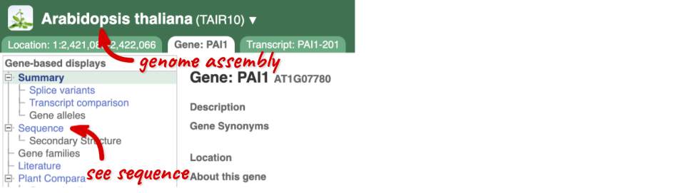
The sequence is shown in FASTA format. The FASTA header contains the genome assembly, chromosome, coordinates and strand (1 or -1) – this gene is on the negative strand.
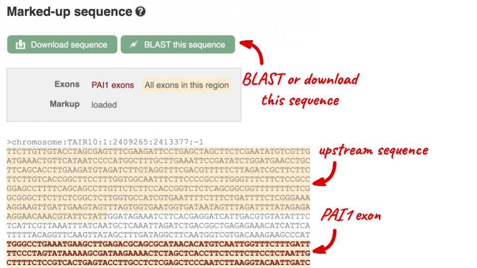
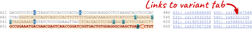
Exons are highlighted within the genomic sequence, both exons of our gene of interest and any neighbouring or overlapping gene. By default, 600 bases are shown up and downstream of the gene. We can make changes to how this sequence appears with the blue Configure this page button found at the left. This allows us to change the flanking regions, add variants, add line numbering and more. Click on it now.

Once you have selected changes (in this example, Show variants and Line numbering) click at the top right.
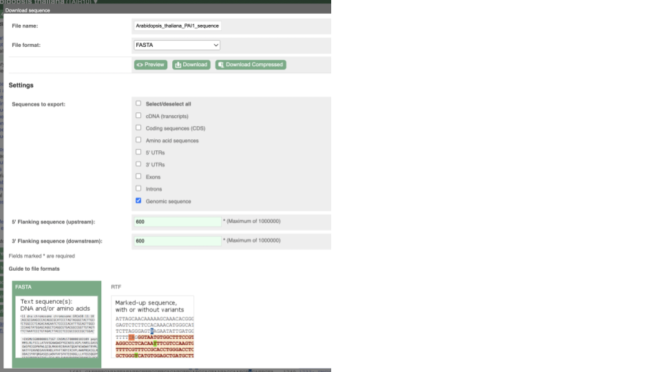
You can download this sequence by clicking in the Download sequence button above the sequence:
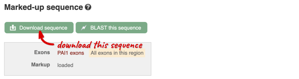
This will open a dialogue box that allows you to pick between plain FASTA sequence, or sequence in RTF, which includes all the coloured annotations and can be opened in a word processor. If you want run a sequence analysis tool, download as FASTA sequence, whereas if you want to analyse the sequence visually, RTF is best for this. This button is available for all sequence views.
To find out what the protein does, have a look at GO terms from the Gene Ontology consortium. There are three pages of GO terms, representing the three divisions in GO: Biological process (what the protein does), Cellular component (where the protein is) and Molecular function (how it does it). Click on GO: Biological process to see an example of the GO pages.
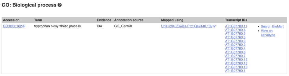
Here you can see the functions that have been associated with the gene. There are three-letter codes that indicate how the association was made, as well as links to the specific transcript they are linked to.
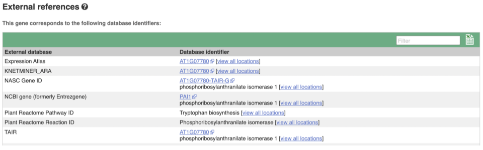
We also have links out to other databases which have information about our genes and may focus on other topics that we don’t cover, like Expression Atlas or UniProtKB. Go up the left-hand menu to External references:
Demo: The transcript tab
We’re now going to explore the different transcripts of PAI1. Click on Show transcript table at the top.
![]()
![]()
Here we can see a list of all the transcripts of PAI1 with their identifiers, lengths and biotypes. Click on the ID of the Ensembl Canonical transcript, PAI1-211.
You are now in the Transcript tab for PAI1-211. We can still see the gene tab so we can easily jump back. The left hand navigation column provides several options for the transcript PAI1-211 - many of these are similar to the options you see in the gene tab, but not all of them. If you can’t find the thing you’re looking for, often the solution is to switch tabs.
Click on the Exons link. This page is useful for designing RT-PCR primers because you can see the sequences of the different exons and their lengths.
![]()
You may want to change the display (for example, to show more flanking sequence, or to show full introns). In order to do so click on Configure this page and change the display options accordingly.
Now click on the cDNA link to see the spliced transcript sequence with the amino acid sequence. This page is useful for mapping between the RNA and protein sequences, particularly genetic variants.
![]()
UnTranslated Regions (UTRs) are highlighted in dark yellow, codons are highlighted in light yellow, and exon sequence is shown in black or blue letters to show exon divides. Sequence variants are represented by highlighted nucleotides and clickable IUPAC codes are above the sequence.
Next, follow the General identifiers link at the left. Just like the External References page in the gene tab, this page shows links out to other databases such as RefSeq, UniProtKB, PDBe and others, this time linked to the transcript or protein product, rather than the gene.
![]()
If you’re interested in protein domains, you could click on Protein summary to view domains from Pfam, PROSITE, Superfamily, InterPro, and more. These are all plotted against the transcript sequence, with the exons shown in alternating shades of purple at the top of the page. Alternatively, you can go to Domains & features to see a table of the same information.
![]()
![]()
Exploring the CCD7 gene in Arabidopsis thaliana
-
Find the Arabidopsis thaliana CCD7 gene on Ensembl Plants. On which chromosome and which strand of the genome is this gene located?
-
Where in the cell is the CCD7 protein located?
-
What is the source of the assigned gene name?
-
How many transcripts does it have? How long is its longest transcript (in bp)? How long is the protein it encodes? How many exons does it have? Are any of the exons completely or partially untranslated?
- Go to the Ensembl Plants homepage (http://plants.ensembl.org/). Select A. thaliana from the species list and type
CCD7in the search box. Click Go and click on the gene ID AT2G44990. You can find the strand orientation and the location under Summary in the Gene tab.The A. thaliana CCD7 gene is located on chromosome 2 on the forward strand.
- Click on GO: Cellular component in the left-hand panel.
The protein is located in the chloroplast and plastid.
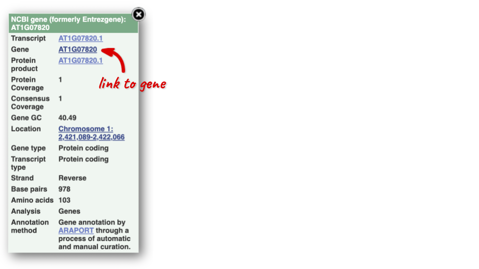
- Click on Summary in the side menu.
The gene name is assigned and imported from NCBI gene (formerly Entrezgene).
- Click on Show transcript table.
There are 3 transcripts. The longest one is 2005 bp and the length of the encoded protein is 622 amino acids.
Click on the transcript ID AT2G44990.3 in the transcript table. You can find the number of exons in under in the summary information at the top of the page.
It has 6 exons.
Click on Sequence: Exons in the left-hand panel.
The first and last exons are partially untranslated (sequence shown in orange). This can also been seen from the fact that in the transcript diagrams on the Gene Summary and Transcript Summary pages the boxes representing the first and last exon are partially unfilled.
Finding a Triticum aestivum gene
-
Search for
Oxygen evolving enhancer proteinfrom the Ensembl Plants homepage and narrow down your search to Triticum aestivum. How many genes are there with this name in wheat? Why do you think this is? What chromosomes are they on? -
Go to the gene on chromosome 2B. How many protein-coding transcripts does this gene have? What is a “canonical transcript”?
-
Click on the canonical transcript. How many exons does this transcript have? Export the protein sequence of this transcript in the FASTA format.
- Start at the Ensembl Plants homepage. Choose Triticum aestivum from the species drop-down, type
Oxygen evolving enhancer proteininto the search box then click Go.There are two genes named TraesCS2D02G248400 and TraesCS2B02G270300. This is because of the hybridisations in wheat’s evolutionary history. You can see that the two genes occur on chromosomes 2B and 2D.
- Click on the gene on chromosome 2B to go to the Gene tab. If the transcript table is hidden, click on Show transcript table to see it.
There are 2 protein coding transcripts.
Mouse over the Ensembl Canonical flag in the transcripts table to find a description.
The Ensembl canonical transcript is a single transcript chosen for each gene in each species. It is the most highly conserved, most highly expressed, has the longest coding sequence and is represented in other key resources (e.g. NCBI, UniProt)
- Click on TraesCS2B02G270300.2 in the transcript table. You can find the number of exons in the summary description at the top of the Summary page, or you can count the number of boxes (boxes represent exons, lines represent introns) in the Summary diagram.
TraesCS2B02G270300.2 has 2 exons.
Go to Sequence: Protein In the left-hand panel.
Click on the green Download sequence button above the protein sequence. Select FASTA from the drop-down in the pop-up menu and download the sequence to your local machine.
BioMart
Follow these instructions to guide you through BioMart to answer the following query:
- What genes are found on chromosome 9, between 15274000 and 15300000 in Oryza sativa Japonica?
- What are the NCBI Gene IDs for these genes?
- Are there associated functions from the GO (gene ontology) project that might help describe their function?
- What are their cDNA sequences?
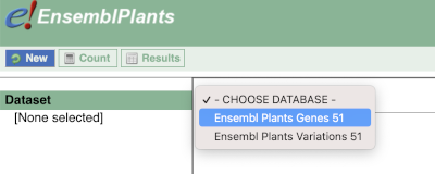
Click on BioMart in the top header of a plants.ensembl.org page to go to: plants.ensembl.org/biomart/martview
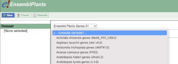
You cannot choose any filters or attributes until you’ve chosen your dataset. Your dataset is the data type you’re working with. In this case we’re going to choose human genes, so pick Ensembl Plants Genes then Oryza sativa Japonica Group genes from the drop-downs.
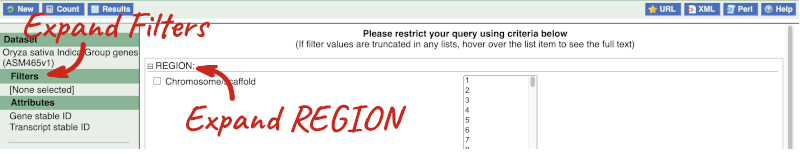
Now that you’ve chosen your dataset, the filters and attributes will appear in the column on the left. You can pick these in any order and the options you pick will appear.
Click on Filters on the left to see the available filters appear on the main page. You’ll see that there are loads of categories of Filters to choose from. You can expand these by clicking on them. For our query, we’re going to expand REGION.
Our input data is a locus, so we’re going to use the chromosome and coordinates filters. Choose chromosome 9 from the drop-down menu and paste in the start and the end coordinates (15274000 and 15300000). The filters will be autoselected when you add values to them and will appear in the left-hand column.
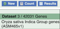
To check if the filters have worked, you can use the Count button at the top left, which will show you how many genes have passed the filter. If you get 0 or another number you don’t expect, this can help you to see if your query was effective.
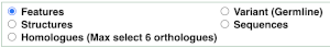
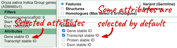
To choose the attributes, expand this in the menu. There are five categories for rice gene attributes. These categories are mutually exclusive, you cannot pick attributes from multiple categories. This means that we need to do two separate queries to get our GO terms and NCBI IDs, and to get our cDNA sequences.
The Ensembl gene and transcript IDs are selected by default. The selected attributes are also listed on the left.
We can choose the attributes we want by clicking on them. For our query, we’re going to select:
- GENE
- Gene Name
- EXTERNAL
- NCBI gene ID
- GO term accession
- GO term name
- GO term definition
We need to select the Gene Name in order to get back our original input, as this is not returned by default in BioMart. The order that you select the attributes in will define the order that the columns appear in in your output table.
You can get your results by clicking on Results at the top left.
The results table just gives you a preview of the first ten lines of your query. This allows the results to load quickly, so that if you need to make any changes to your query, you don’t waste any time. To see the full table you can click on View ## rows. You can also export the data to an xls, tsv, csv or html file. For large queries, it is recommended that you export your data as Compressed web file (notify by email), to ensure your download is not disrupted by connection issues.
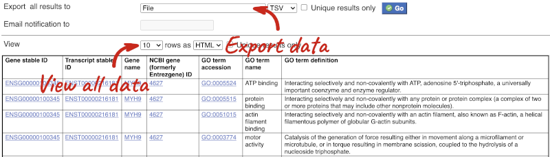
You can see multiple rows per gene in your input list, because there are multiple transcripts per gene and multiple GO terms per transcript.
To get the cDNA sequences, go back to the Attributes then select the category Sequences and expand SEQUENCES.
When you select the sequence type, the part of the transcript model you’ve chosen will be highlighted in the grpahic.
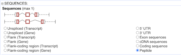
Choose cDNA sequences, then expand HEADER INFORMATION to add Gene Name to the header. Then hit Results again.
For more details on BioMart, have a look at this publication:
Kinsella, R.J. et al
Ensembl BioMarts: a hub for data retrieval across taxonomic space.
http://europepmc.org/articles/PMC3170168
Ensembl Plants: finding genes by protein domain
One class of disease resistance (R) genes in plants are the TIR-NBS-LRR genes, that code for proteins that contain an N-terminal Toll/Interleukin receptor homology region (TIR), a nucleotide binding site (NBS) and a C-terminal leucine rich repeat (LRR). TIR-NBS-LRR genes are common in dicots but seem to be rare in monocots (Tarr and Alexander. TIR-NBS-LRR genes are rare in monocots: evidence from diverse monocot orders. BMC Res Notes 2009 Sep 8;2:197).
The ID for the TIR domain in the Pfam (protein family) database is PF01582.
Use BioMart in Ensembl Plants to generate a list of all Solanum tuberosum (potato; a dicot) genes that are annotated to contain a TIR domain. Include the Ensembl stable ID and gene description. Do the same for Zea mays (maize; a monocot).
Do your results confirm the findings of Tarr and Alexander?
-
Go to Ensembl Plants and click on the link Tools at the top of the page. Click on BioMart. Choose the Ensembl Plants Genes database. Choose the Solanum tuberosum genes dataset.
- Now, filter for the genes containing a TIR domain: Click on Filters in the left panel. Expand the PROTEIN DOMAINS AND FAMILIES section. Select Limit to genes with these family or domain IDs and enter
PF01582in the box. Select Pfam ID(s) (e.g. PF00004) from the drop-down menu. Click on Count in the toolbar.This should give you 78 / 40336 genes.
-
Specify the attributes to be included in the output (note that a number of attributes will already be selected by default). Click on Attributes in the left panel. Expand the GENE section. Deselect Transcript stable ID. Select Gene description.
-
Now click on Results. The first 10 results are displayed by default. You can display all results by selecting View: All rows from the drop-down menu. If you prefer, you can also export as a CSV, TSV or XLS file by using the Export all results to option.
Repeat the above for the Z. mays genes (B73 RefGen_v4) dataset.
Your results should show 3 / 44303 genes containing a TIR domain for maize. The results confirm the findings of Tarr and Alexander.
Mapping Uniprot IDs in Ensembl Plants
BioMart is a very handy tool when you want to map between different databases. The following is a list of IDs from the UniProtKB/Swiss-Prot database of Arabidopsis thaliana proteins that are supposedly involved in flavonoid metabolism: P42813, Q9LS08, Q9ZST4, Q9SYM2, P51102, Q9LPV9, Q9FE25, Q96323, Q9FKW3, P13114, P41088, Q9S818, Q96330, O22203, Q39224, O22264, Q9SD85, Q9LYT3, Q9FJA2, Q43128, P43254, O04153, Q43125, Q9S9P6, Q94C57, Q9LNE6, Q9FK25, Q9SYM5, Q9ZQ95
Using BioMart in Ensembl Plants a list that shows to which Ensembl Gene IDs these UniProtKB/Swiss-Prot IDs map. Also include the gene name and description.
-
Go to BioMart in Ensembl Plants. Click the New button on the toolbar in the top left-hand corner to start a new query. Choose the Ensembl Plants Genes database. Choose the Arabidopsis thaliana genes dataset.
-
Click on Filters in the left panel. Expand the GENE section. Select ID list limit – UniProt/Swissprot ID(s). Enter the list of IDs in the text box (either comma separated or as a list).
-
Click on Attributes in the left panel. Expand the GENE section. Deselect Transcript Stable ID. Select Gene name and Gene description. Expand the EXTERNAL section. Select UniProtKB/SwissProt ID(s).
-
Click the Results button on the toolbar. Select View: All rows as HTML or export all results to a file. Tick the box Unique results only.
Your results should show 28 / 32833 genes.
Mapping microarray probes to genes
The following is a list of 101 probes that were upregulated after short-term phosphate deprivation of Arabidopsis thaliana. The microarray used was the Arabidopsis thaliana whole genome Affymetrix gene chip (ATH1) (Misson et al. A genome-wide transcriptional analysis using Arabidopsis thaliana Affymetrix gene chips determined plant responses to phosphate deprivation. Proc Natl Acad Sci U S A. 2005 August 16; 102(33): 11934–11939).
259842_at, 251193_at, 259303_at, 252534_at, 266957_at, 257891_at, 263593_at, 266372_at, 265342_at, 254011_at, 260623_at, 262238_at, 264118_at, 256910_at, 263846_at, 249996_at, 248094_at, 267361_at, 246275_at, 258034_at, 248622_at, 263483_at, 254250_at, 257964_at, 248566_s_at, 245263_at, 264636_at, 264342_at, 254125_at, 262369_at, 259399_at, 251770_at, 266132_at, 246001_at, 246075_at, 258887_at, 258856_at, 263391_at, 256376_s_at, 266766_at, 258277_at, 266142_at, 246071_at, 261021_at, 251143_at, 252730_at,249337_at, 258158_at, 245882_at, 250054_at, 263539_at, 263851_at, 247949_at, 262229_at, 246777_at, 258975_at, 247026_at, 252265_at, 256100_at, 246099_at, 246302_at, 254111_at, 256017_at, 259750_at, 254215_at, 253271_s_at, 247314_at, 267567_at, 250435_at, 255543_at, 259479_at, 264783_at, 245193_at, 260561_at, 263948_at, 258682_at, 253386_at, 263847_at, 266017_at, 252414_at, 255360_at, 251176_at, 266743_at, 253829_at, 267497_at, 258613_at, 253163_at, 261648_at, 258100_at, 249983_at, 266413_at, 264261_at, 256627_at, 249640_at, 248164_at, 266184_s_at, 247047_at, 263083_at, 251961_at, 252011_at, 260101_at
(a) Generate a list of the genes to which these probesets map. Include the Ensembl Gene ID, name, description and probe ID attributes.
(b) As a first step in order to be able to analyse them for possible regulatory features they have in common, retrieve the 250 bp upstream of the transcripts of these genes. Include the Ensembl Gene ID, name and description attributes in the sequence header.
(a) Click the New button on the toolbar. Choose the Ensembl Plants Genes database. Choose the Arabidopsis thaliana genes dataset.
Click on Filters in the left panel. Expand the GENE section. Select Input microarray probes/probesets ID list – Affymetrix array Arabidopsis ATH1 121501 ID(s). Enter the list of probeset IDs in the text box (either comma separated or as a list). Click the Count button on the toolbar.
Click on Attributes in the left panel. Expand the GENE section. Deselect Transcript Stable ID. Select Gene name and Gene description. Expand the EXTERNAL section. Select Affymetrix array Arabidopsis ATH1 121501.
Click the Results button on the toolbar. Select View All rows as HTML or export all results to a file. Tick the box Unique results only.
Your results should show 104 / 32833 genes. Apparently there are a few probes that have been mapped to more than one gene.
(b) You can leave the dataset and filters the same, so you can directly specify the attributes:
Click on Attributes in the left panel. Select the Sequences attributes page. Expand the SEQUENCES section. Select Flank (Transcript). Enter 250 in the Upstream flank text box. Expand the HEADER INFORMATION section. Select, in addition to the default selected attributes, Gene name and Gene description.
Note: Flank (Transcript) will give the flanks for all the transcripts of a gene with multiple transcripts. Flank (Gene) will give the flank for the transcript with the outermost 5’ (or 3’) end.
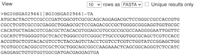
Click the Results button on the toolbar. Select View All rows as FASTA or export all results to a file.
Custom data
Demo: Upload small files
We have some Arabidopsis mutants characterised by increased plant branching. They all have large scale deletions on chromosome one:
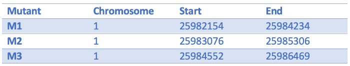
We can turn them into a BED file and view them in the genome browser:
chr1 25982154 25984234 M1
chr1 25983076 25985306 M2
chr1 25984552 25986469 M3
You can add data from a Region in Detail page by clicking on the Custom tracks button at the left. Alternatively, go to a species homepage and click on Display your data in Ensembl Plants.

A menu will appear:
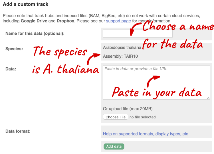
The interface detects file types if you upload or attach a file. When you paste in your data, it can’t do this so we have to tell it what our file type is. It will give you an option where you can select BED.
Click Add data.
You should get to a dialogue box telling you your upload has been successful.
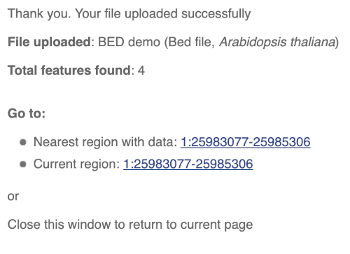
Click on the genomic coordinates link to go to the nearest region with data.
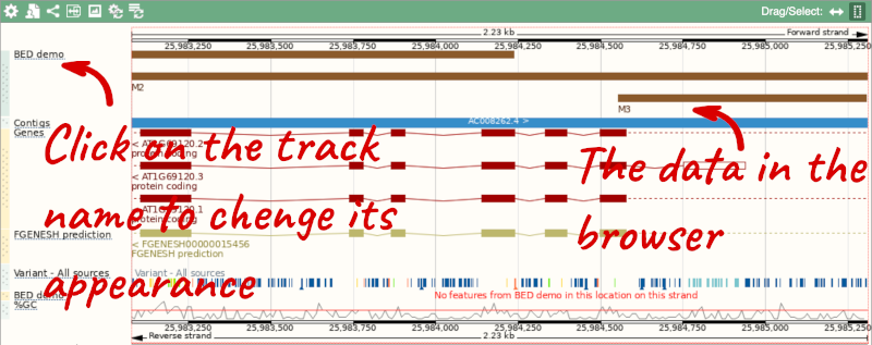
To have a look at the file, click on Custom tracks.
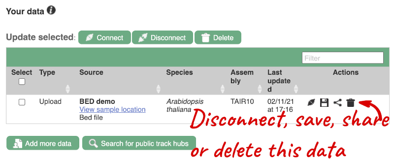
If you’ve got an Ensembl account, you can save this data to your account. Accounts are free to set up and allow you to save configurations and data, and share with groups. You can also permanently delete or temporarily disconnect data from here.
Demo: Attach URLs of large files
Larger files, such as BAM files generated by NGS, need to be attached by URL. You can find seedling RNAseq reads from the 19 genomes project aligned to the Arabidopsis thaliana assembly here: http://mtweb.cs.ucl.ac.uk/mus/www/19genomes/RNA.seedlings.BAM/v9/Col_0.R1.9.bam
Let’s take a look at the folder.
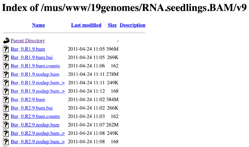
Here you can see a number of BAM files (.bam) with corresponding index files (.bam.bai). We’re interested in the files Col_0.R1.9.bam and Col_0.R1.9.bam.bai. These files are the BAM file and the index file respectively. When attaching a BAM file to Ensembl, there must be an index file in the same folder.
To attach the file, click on Custom tracks, then click on Add more data to add a new track.
We get to the same dialogue box as before. This time we’ll name our data RNAseq reads.
Paste in the URL of the BAM file itself (http://mtweb.cs.ucl.ac.uk/mus/www/19genomes/RNA.seedlings.BAM/v9/Col_0.R1.9.bam).
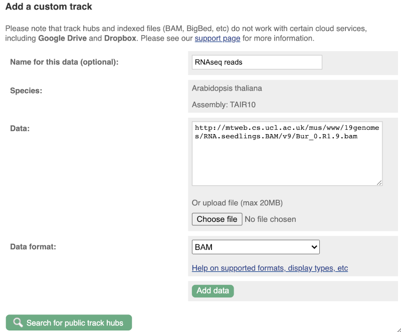
Since this is a file, the interface is able to detect the “.BAM” file extension, so automatically labels the format as BAM. Click on Add data. You should get to a dialogue box telling you your data has been attached successfully. Close the menu to go back to your region of interest.
Let’s go to the region of the AT1G51745 gene. Search for the gene using the Gene text box and click Go.
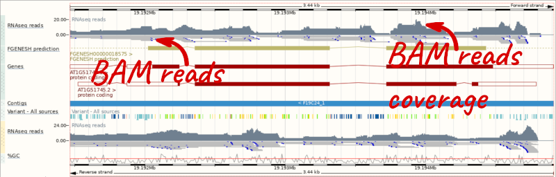
We can zoom in to see the sequence itself. Drag out boxes in the view to zoom in, until you see a view like this. Alternatively, type 1:19194595-19194630 in the Location box and clicking Go to jump to a smaller region.
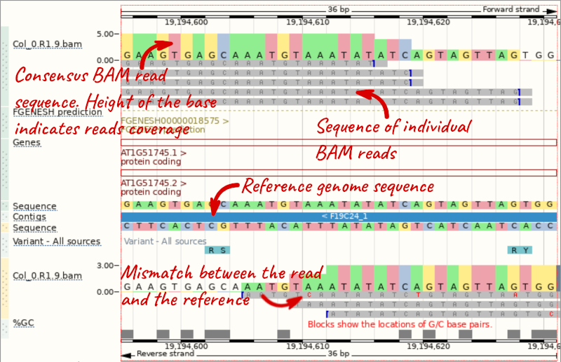
Any mismatches between the reads and the reference genome assembly are shown in red.
Demo: Track hub registry
Track Hub Registry provides publicly available data organised in track hubs. Ensembl established a pipeline for generating track hubs for all public RNA-Seq studies in the INSDC archives. This pipeline discovers and aligns reads from RNA-Seq studies across all plant species in Ensembl Plants, which means that you can search the Track Hub Registry for available RNA-Seq data and display them in the genome browser.
You can search for track hubs to add in different ways:
- Search for track hubs in the Track Hub Registry and choose to add them to your genome browser of choice.
- Search the track hub registry using the Track Hub Registry interface in Ensembl Plants (there is a link from the homepage).
We will now add the track hub containing data on epigenetic regulation of transcription initiation in Arabidopsis (DRP006159).
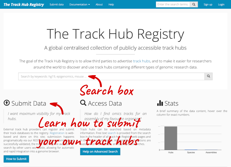
You can add track hubs to view in Ensembl directly via the Track Hub Registry. Go to the Track Hub Registry homepage and search for DRP006159.
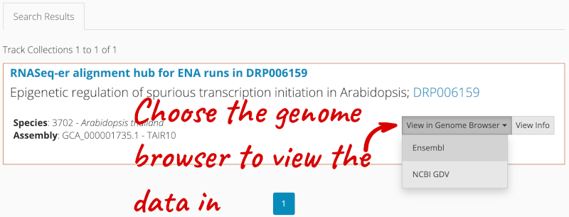
There is one RNA-seq alignment hub returned, which you can view in the genome browser.
Alternatively, you can add track hubs by searching the Track Hub Registry through Ensembl. Click the Custom tracks -> Track Hub Registry Search in any region view within Ensembl.
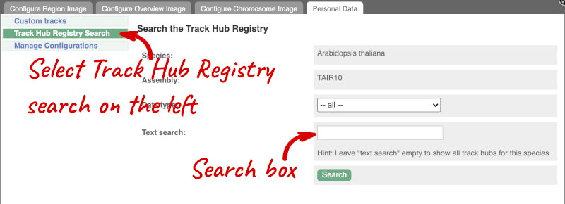
You can only find track hubs for the selected species and assembly denoted in the search box.
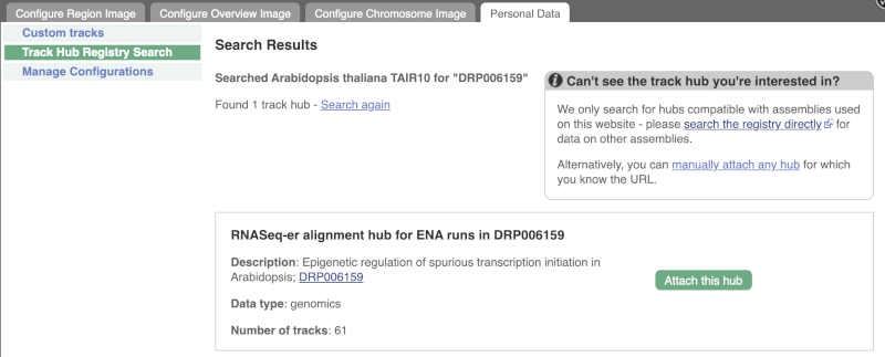
Search for DRP006159.
Click Attach this hub in the search results page.
Track Hubs often contain vast amounts of data, which can slow Ensembl down, so only add them if you need them, and trash them when you are finished with them.
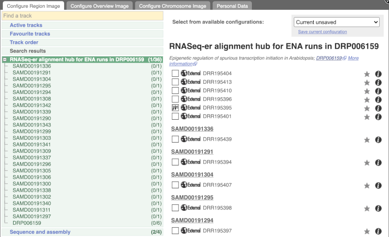
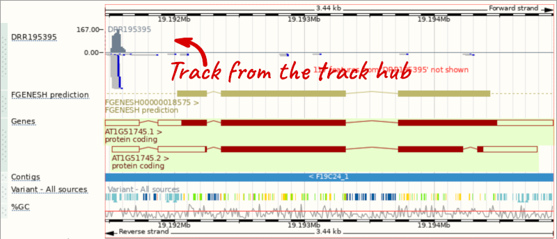
Go to Configure this Page to see that a new category has been added to your menu. Add track for the DRR195395 run to the Region in Detail view by ticking the box.
This data represents genome-wide map of transcription start sites (TSSs) in A. thaliana mutants generated using CAGE-seq. Can you see the high reads coverage corresponding to the TSS of our AT1G51745 gene?
Viewing gene features on the Arabidopsis karyotype
Here is a list of several genes linked to regulation of long-day photoperiodism in Arabidopsis thaliana.
AGL17, APRF1, CDF5, CDKD-2, CLF, COL9, EBS, EFM, ELF6, GI, JMJ14, LATE, MED16, MRG1, MRG2, MYB56, NFYC4, PEP, POL2A, SHW1, VOZ1, VOZ2
(a) Can you display these Arabidopsis genes on the karyotype? Can you find the location for all of these genes?
(b) Can you export this image?
(c) How can you delete this data?
(a) Go to Ensembl Plants, choose Arabidopsis thaliana and click on View karyotype. Click on + Add features and enter the list of genes. You can also customise the pointer style. Click on Show features once ready. You will see the karyotype with the locations of the genes shown as little triangles. The table provides additional information on the genes displayed on the karyotype. You may want to explore some of those links and view the genes on their Location tabs. These genes are scattered on all Arabidopsis autosomes (chromosomes one to five).
(b) You can export the image by clicking on the polaroid photo icon at the top bar in the image you want to export. This functionality is available throughout the Ensembl browser.
(c) Once in the karyotype view, click on Custom data in the side menu. You can delete the gene features on the Arabidopsis karyotype by clicking on the rubbish bin next to Gene track.
Adding Wiggle files to Ensembl Plants
Upload the ZM_wiggle.wig file to the Zea mays genome in Ensembl Plants. View this track across the region 1:2884000-2898000. What is the highest score in this region?
Go to Ensembl Plants and click on Zea mays to go to the species homepage.
Select Display your data in Ensembl Plants to get to the custom track menu. Select Choose file and select the file location. The file type should be automatically selected. Click Add data.
Click on the Nearest region with data in the results page. From the region page you reach, put the coordinates 1:2884000-2898000 into the Location box to jump to the region.
The highest score is 99 and it overlaps the GRMZM2G086269 gene.
Adding track hubs to Ensembl Plants
(a) How many publicly available track hubs are there for the Solanum lycopersicum genome?
(b) Add the RNASeq-er alignment hub for ENA runs in ERP022223 track hub containing Illumina RNA-seq data of tomato roots colonized by the plant growth-promoting rhizobacterium Pseudomonas fluorescens strain CREA-C16. Search for Solyc07g065860.3, a tomato orthologue of the Arabidopsis RGI3 gene involved in regulation of root development root meristem growth. Is this gene expressed?
(c) Go to the region 7:67591664-67591688. Can you see any mismatches between reads and the reference assembly? Are they real SNPs or sequencing errors?
Go to Ensembl Plants and click on View full list of all species. Search the table for Solanum lycopersicum. Click on the species name to go to the species homepage.
Select Display your data in Ensembl Plants to get to the custom track menu, then click on Track Hub Registry Search in the side panel. Hit Search to find all available track hubs.
There are 315 track hubs currently available for tomato.
Click Search again at the top of the page and type ERP022223 in the provided text search box. Click Search, then Attach this hub in the search results and close the window by clicking on the tick. Search for Solyc07g065860.3 in the search box. Click on the location coordiantes to go to the Location tab.
This gene is expressed as indicated by the high coverage of RNAseq reads mapping to this locus.
From the region page, put the coordinates 7:67591664-67591688 into the Location box.
There are 11 mismatches between the reads and the genome assembly indicated in red. They represent sequencing errors, as they are found in single reads and concentrate around the read ends.