Filter Events by Year
Ensembl Browser Workshop - EuroFAANG AQUA-FAANG workshop: methods to use and reuse the AQUA-FAANG data and Ensembl resources to advance science
Course Details
- Lead Trainer
- Aleena Mushtaq
- Event Dates
- 2023-04-17 until 2023-04-18
- Location
- Virtual: EMBL-EBI, Hinxton
- Description
- Work with the Ensembl Outreach team to get to grips with the Ensembl browser, accessing and analysing genomic data from fish species represeted in the AQUA-FAANG project.
- Survey
- Ensembl Browser Workshop - EuroFAANG AQUA-FAANG workshop: methods to use and reuse the AQUA-FAANG data and Ensembl resources to advance science Feedback Survey
Demos and exercises
Ensembl species
The front page of Ensembl is found at ensembl.org. It contains lots of information and links to help you navigate Ensembl:
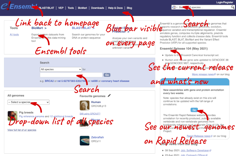
At the top left you can see the current release number and what has come out in this release. To access old releases, scroll to the bottom of the page and click on View in archive site.
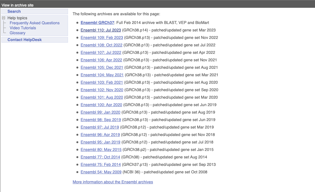
Click on the links to go to the archives. Alternatively, you can jump quickly to the correct release by putting it into the URL, for example e105.ensembl.org jumps to release 105.
Click on View full list of all species.
Click on the common name of your species of interest to go to the species homepage. We’ll click on Atlantic Salmon.
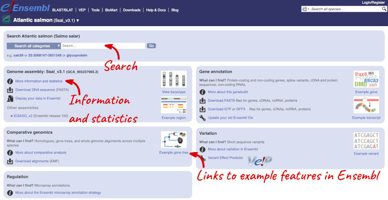
Here you can see links to example pages and to download flatfiles. To find out more about the genome assembly and genebuild, click on More information and statistics.
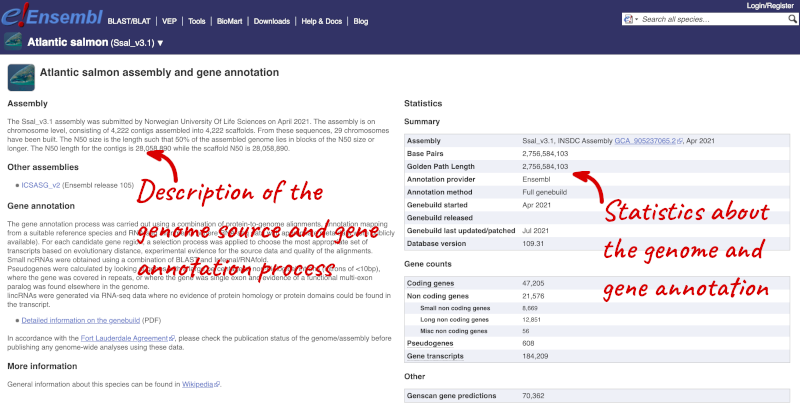
Here you’ll find a detailed description of how to the genome was produced and links to the original source. You will also see details of how the genes were annotated.
Turbot genome assembly
-
Go to the species homepage for Turbot. What is the name of the genome assembly for Turbot?
-
How long is the Turbot genome (in bp)? How many genes have been annotated?
- Select Turbot from the drop down species list, or click on View full list of all Ensembl species, then choose Turbot from the list.
The assembly is ASM1334776v1 or GCA_013347765.1. - Click on More information and statistics. Statistics are shown in the tables on the left.
The length of the genome is 556,696,898 bp.
There are 21,263 coding genes.
Available European seabass assemblies
What previous assemblies are available for European seabass?
Navigate to the Ensembl Homepage (www.ensembl.org). Navigate to the European seabass species homepage by clicking on ‘View full list of all species’, filtering the table of species by searching for European seabass and clicking on the species name within the table. Under Other assemblies one previous assembly and the release you can find it in is listed.
Assembly seabass_V1.0 is available in the archived Ensembl 105 release.
Exploring Genomic Regions
Start at the Ensembl front page, ensembl.org. You can search for a region by selecting your species of interest form the drop-down menu and typing the coordinates into the search box.
To search for a genomic region, you need to input your region coordinates in the correct format, which is chromosome, colon, start coordinate, dash, end coordinate, with no spaces for example: 25:4274500-4302000. Type (or copy and paste) these coordinates into the search box.
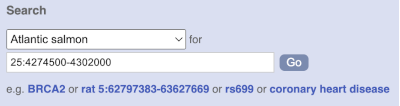
Press Enter or click Go to jump directly to the Region in detail Page.
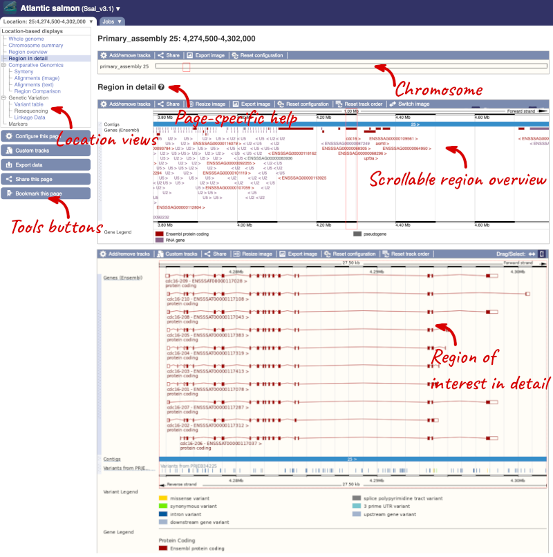
Click on the  button to view page-specific help. The help pages provide text, labelled images and, in some cases, help videos to describe what you can see on the page and how to interact with it.
The Region in detail page is made up of three images, let’s look at each one in detail.
The first image shows the chromosome:
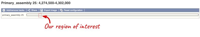
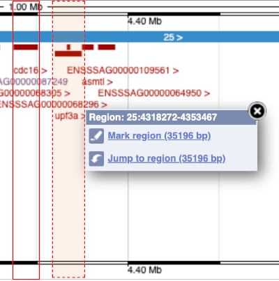
The region we’re looking at is highlighted on the chromosome. You can jump to a different region by dragging out a box in this image. Drag out a box on the chromosome, a pop-up menu will appear.
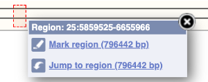
If you wanted to move to the region, you could click on Jump to region (### bp). If you wanted to highlight it, click on Mark region (###bp). For now, we’ll close the pop-up by clicking on the X on the corner.
The second image shows a 1Mb region around our selected region. This is always 1Mb in human, but the fixed size of this view varies between species. This view allows you to scroll back and forth along the chromosome.
You can also drag out and jump to or mark a region.
Click on the X to close the pop-up menu.
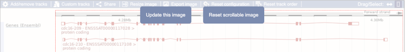
Click on the Drag/Select button  to change the action of your mouse click. Now you can scroll along the chromosome by clicking and dragging within the image. As you do this you’ll see the image below grey out and two blue buttons appear. Clicking on Update this image would jump the lower image to the region central to the scrollable image. We want to go back to where we started, so we’ll click on Reset scrollable image.
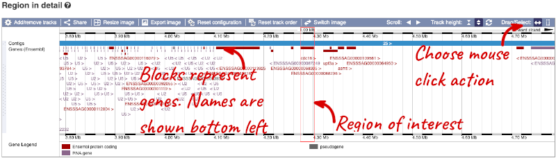
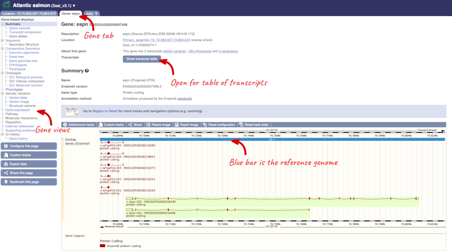
The third image is a detailed, configurable view of the region.
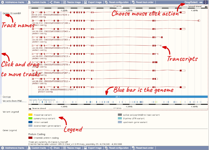
Here you can see various tracks, which is what we call a data type that you can plot against the genome. Some tracks, such as the transcripts, can be on the forward or reverse strand. Forward stranded features are shown above the blue contig track that runs across the middle of the image, with reverse stranded features below the contig. Other tracks, such as variants, regulatory features or conserved regions, refer to both strands of the genome, and these are shown by default at the very top or very bottom of the view.
You can use click and drag to either navigate around the region or highlight regions of interest, Click on the Drag/Select option at the top or bottom right to switch mouse action. On Drag, you can click and drag left or right to move along the genome, the page will reload when you drop the mouse button. On Select you can drag out a box to highlight or zoom in on a region of interest.
With the tool set to Select, drag out a box around an exon and choose Mark region.
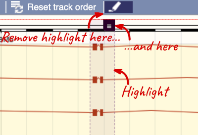
The highlight will remain in place if you zoom in and out or move around the region. This allows you to keep track of regions or features of interest.
We can edit what we see on this page by clicking on the blue Configure this page menu at the left.

This will open a menu that allows you to change the image.
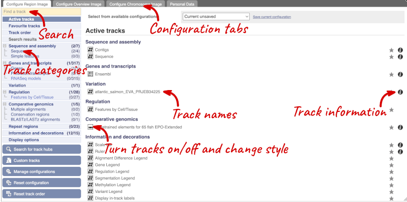
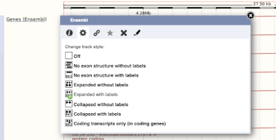
There are thousands of possible tracks that you can add. When you launch the view, you will see all the tracks that are currently turned on with their names on the left and an info icon on the right, which you can click on to expand the description of the track. Turn them on or off, or change the track style by clicking on the box next to the name. More details about the different track styles are in this FAQ: http://www.ensembl.org/Help/Faq?id=335.
You can find more tracks to add by either exploring the categories on the left, or using the Find a track option at the top left. Type in a word or phrase to find tracks with it in the track name or description.
Let’s add some tracks to this image. Add:
- Repeats (Teleost)
- RNASeq models - Heart - BAM files (Unlimited) and Gene models (Expanded with labels)
Now click on the tick in the top left hand to save and close the menu. Alternatively, click anywhere outside of the menu. We can now see the tracks in the image. The proteins track is stranded, so you will see two tracks, one above and one below the contig, representing the proteins mapped to the forward and reverse strands respectively. The variants track is not stranded, so is found near the bottom of the image.
If the track is not giving you can information you need, you can easily change the way the tracks appear by hovering over the track name then the cog wheel to open a menu. To make it easier to compare information between tracks, such as spotting overlaps, you can move tracks around by clicking and dragging on the bar to the left of the track name.
Now that you’ve got the view how you want it, you might like to show something you’ve found to a colleague or collaborator. Click on the Share this page button to generate a link. Email the link to someone else, so that they can see the same view as you, including all the tracks you’ve added. These links contain the Ensembl release number, so if a new release or even assembly comes out, your link will just take you to the archive site for the release it was made on.

To return this to the default view, go to Configure this page and select Reset configuration at the bottom of the menu.
Exploring a genomic region in Rainbow trout
-
Go to the region from 49,000,000 to 49,400,000 bp on Rainbow trout chromosome 3.
-
Zoom in on the myo3b gene.
-
Configure this page to turn on the CpG islands track in this view. What tool was used to annotate the CpG islands according to the track information? How many CpG islands can you see within the myo3b gene?
-
Create a Share link for this display. Email it to your neighbour. Open the link they sent you and compare. If there are differences, can you work out why?
-
Export the genomic sequence of the region you are looking at in FASTA format.
-
Turn off all tracks you added to the Region in detail page.
-
Go to the Ensembl homepage. Select Rainbow trout from the Species drop-down list and type
3:49000000-49400000in the text box. Click Go. -
Draw with your mouse a box encompassing the myo3b transcripts. Click on Jump to region in the pop-up menu.
- Click Configure this page in the side menu (or on the cog wheel icon in the top left hand side of the bottom image). Go into Simple features in the left-hand menu then select CpG islands. Click on the (i) button to find out more information.
The CpG islands are determined from the genomic sequence using a program written by G. Micklem, similar to newcpgreport in the EMBOSS package. Save and close the new configuration by clicking on ✓ (or anywhere outside the pop-up window). There is one CpG island overlapping myo3b.
-
Click Share this page in the side menu. Copy the URL. Get your neighbour’s email address and compose an email to them, paste the link in and send the message. When you receive the link from them, open the email and click on your link. You should be able to view the page with the new configuration and data tracks they have added to in the Location tab. You might see differences where they specified a slightly different region to you, or where they have added different tracks.
-
Click Export data in the side menu. Leave the default parameters as they are (FASTA sequence should already be selected). Click Next>. Click on Text. Note that the sequence has a header that provides information about the genome assembly (USDA_OmykA_1.1), the chromosome, the start and end coordinates and the strand. For example:
>3 dna:primary_assembly primary_assembly:USDA_OmykA_1.1:3:49195318:49199101:1 - Click Configure this page in the side menu. Click Reset configuration. Click ✓.
Exploring a genomic region in Gilthead seabream
-
Go to the region from 9,205,000 to 9,554,000 bp on Gilthead seabream chromosome 16.
-
Zoom in on the slc25a21 gene.
-
Configure this page to turn on the RefSeq GFF3 annotation import track in this view. What are the differences between the slc25a1 transcripts annotated by Ensembl and NCBI RefSeq?
-
Go to the Ensembl homepage. Select Gilthead seabream from the Species drop-down list and type
16:9205000-9554000in the text box. Click Go. -
Draw with your mouse a box encompassing the slc25a21 transcripts. Click on Jump to region in the pop-up menu.
-
Click Configure this page in the side menu (or on the cog wheel icon in the top left hand side of the bottom image). Go into Genes in the left-hand menu then select RefSeq GFF3 annotation import. Save and close the new configuration by clicking on ✓ (or anywhere outside the pop-up window).
There are two slc25a21 transcripts annotated by NCBI RefSeq, but three transcripts annotated by Ensembl. The coding sequences of the two transcripts annotated by NCBI RefSeq are the same as the slc25a21-202 transcript (ENSSAUT00010071831.1), with differences in the length of the 5’ and 3’ UTRs. slc25a21-201 (ENSSAUT00010071830.1) has a different exon structure for its final exon, with an extended coding sequence and 3’ UTR.
Genes and Transcripts
Demo: The gene tab
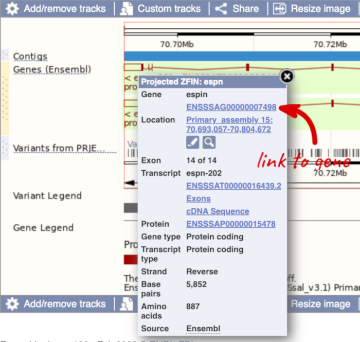
If you click on any one of the transcripts in the Region in detail image, a pop-up menu will appear, allowing you to jump directly to that gene or transcript.
Another way to go to a gene of interest is to search directly for it.
We’re going to look at the Atlantic salmon espn gene. This gene encodes a multifunctional actin-bundling protein with a major role in mediating sensory transduction in various mechanosensory and chemosensory cells.
From ensembl.org, type espn into the search bar and click the Go button. You will get a list of hits with the human gene at the top.
Where you search for something without specifying the species, or where the ID is not restricted to a single species, the most popular species will appear first, in this case, human, mouse and zebrafish appear first. You can restrict your query to species or features of interest using the options on the left.
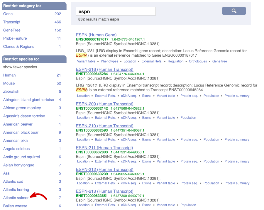
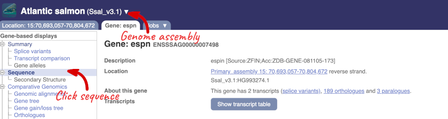
Click on the gene name of the Atlantic salmon. The Gene tab should open:
Let’s walk through some of the links in the left hand navigation column. How can we view the genomic sequence? Click Sequence at the left of the page.
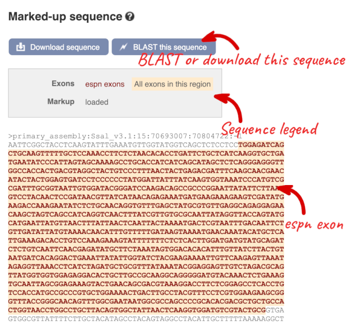
The sequence is shown in FASTA format. Take a look at the FASTA header:

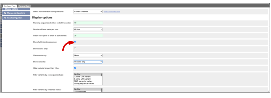
Exons are highlighted within the genomic sequence. Variants can be added with the Configure this page link found at the left. Click on it now.
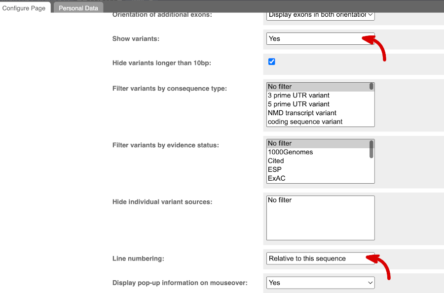
Once you have selected changes (in this example, Show variants and Line numbering: Relative to this sequence) click at the top right.
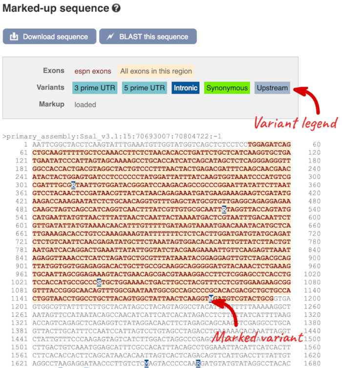
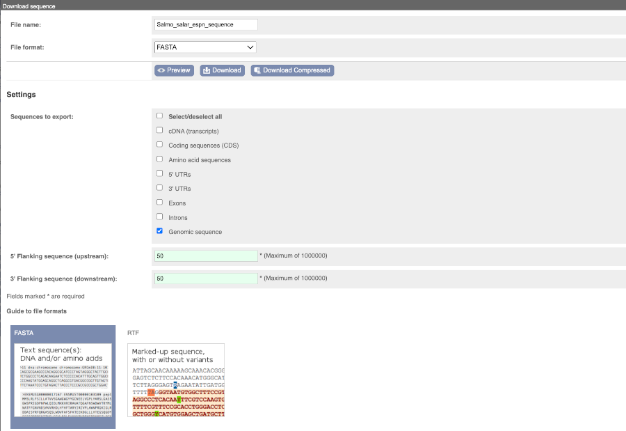
You can download this sequence by clicking in the Download sequence button above the sequence:

This will open a dialogue box that allows you to pick between plain FASTA sequence, or sequence in RTF, which includes all the coloured annotations and can be opened in a word processor. This button is available for all sequence views.
Can our gene be found in other databases? Go up the left-hand menu to External references:
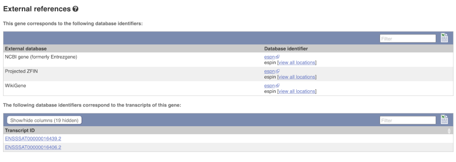
This contains links to the gene in other projects, such as NCBI Gene, and papers where this sequence is published.
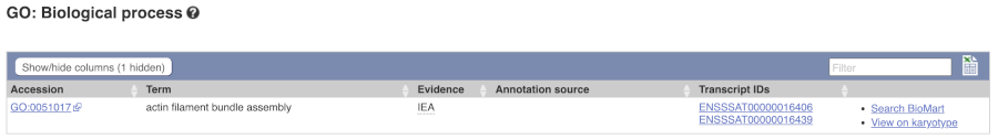
To find out what the protein does, click on GO:biological process to see GO terms from the Gene Ontology consortium.
Demo: The transcript tab
Let’s now explore one splice isoform. Click on Show transcript table at the top.

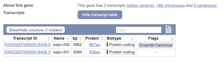
Click on the ID for espn-202, ENSSSAT00000016439.2.
You are now in the Transcript tab for espn-202. The left hand navigation column provides several options for the transcript espn-202.
For detailed information on the support for this transcript, click on Supporting evidence
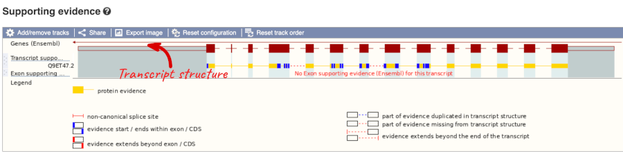
Click on the identifiers of the evidence to get a pop-up. This links out to the original records of these data in, for example, RefSeq, Uniprot or ENA.
Click on the Exons link.
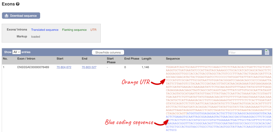
You may want to change the display (for example, to show more flanking sequence, or to show full introns). In order to do so click on Configure this page and change the display options accordingly.
Now click on the cdna link to see the spliced transcript sequence.
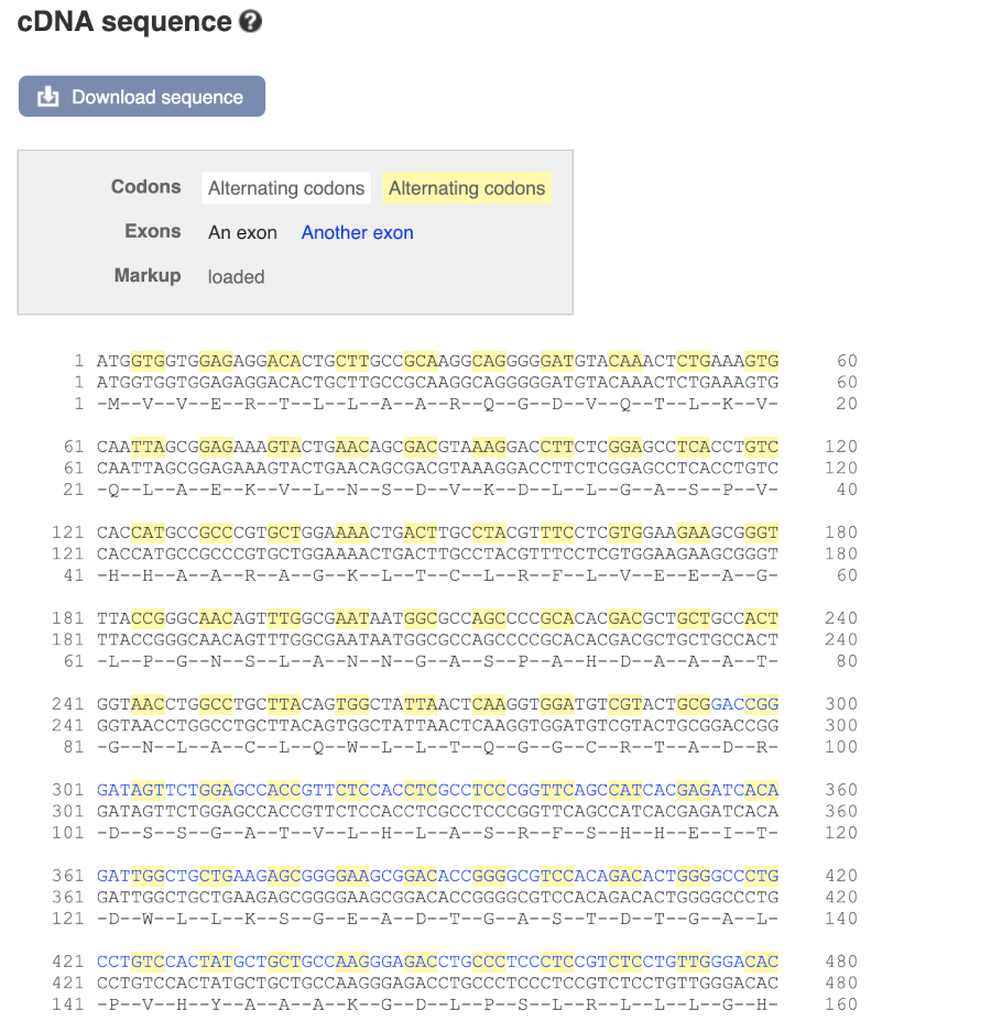
UnTranslated Regions (UTRs) are highlighted in dark yellow, codons are highlighted in light yellow, and exon sequence is shown in black or blue letters to show exon divides.
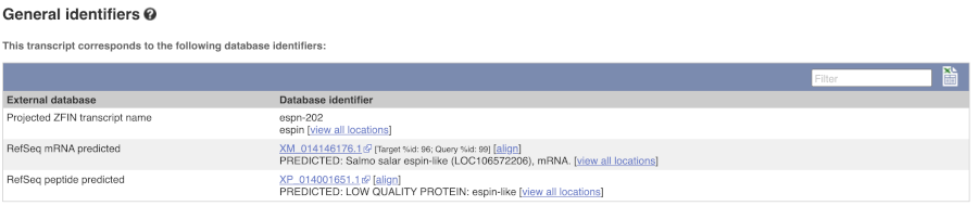
Next, follow the General identifiers link at the left.
This page shows information from other databases such as RefSeq, UniProtKB and others, that match to the Ensembl transcript and protein.
Now click on Protein summary to view domains from Pfam, PROSITE, Superfamily, Panther, and more.
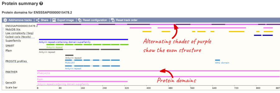
Clicking on Domains & features shows a table of this information.
Exploring the Common carp prkci gene
Search for the Common carp gene prkci.
(a) What GO: biological process terms are associated with the prkci gene?
(b) Go to the transcript tab for the prkci-207 (ENSCCRT00000153471.1) protein coding transcript. How many exons does it have? Which one is the longest? How much of that is coding?
(c) How many different domain prediction methods predict a PB1 domain? Where in the protein is this domain?
(a) Go to the Ensembl homepage (http://www.ensembl.org).
Select Search: Common carp and type prkci. Click Go. Click on the gene link ENSCCRG00000007495.2.
Click on GO: biological process in the side menu. Protein phosphorylation and establishment or maintenance of cell polarity are listed as GO: Biological processes associated with this gene.
(b) Click on the transcript prkci-207 (ENSCCRT00000153471.1). Click on Exons in the left hand menu. There are eighteen exons. Exon 18 is longest with 1,572bp, of which around 88 are coding.
(c) Click on either Protein Summary or Domains & features in the left hand menu to see graphically or as a table respectively. The PB1 domain is predicted by SuperFamily, SMART, Pfam and PROSITE. It is towards the N-terminus of the protein. Clicking on the predicted PB1 domain will open a pop-up window that shows you the amino acid coordinates for the predicted domain.
Exploring the Turbot pcsk2 gene
(a) Find the Turbot pcsk2 (proprotein convertase subtilisin/kexin type 2) gene, and go to the Gene tab.
- On which chromosome and which strand of the genome is this gene located?
- How many transcripts (splice variants) are there and how many are protein coding?
- How long is the protein encoded by ENSSMAT00000034168.2?
- What are some functions of pcsk2 according to the Gene Ontology consortium?
(b) In the transcript table, click on the transcript ID for pcsk2-201, and go to the Transcript tab.
- How many exons does it have?
- Are any of the exons completely or partially untranslated?
(c) Is there any supporting evidence present for ENSSMAT00000034168.2?
(a) Go to the Ensembl homepage.
Select Search: Turbot and type pcsk2. Click Go.
Click on the Ensembl ID ENSSMAG00000020650.
- Chromosome 15 on the reverse strand.
- Ensembl has five protein coding transcripts annotated for this gene.
- It codes for a protein of 629 amino acids
Click on GO:molecular function to see that serine-type endopeptidase activity and serine-type peptidase activity are associated with pcsk2.
(b) Click on ENSSMAT00000034168.2.
It has thirteen exons. This is shown in the Transcript summary or in the left hand side menu Exons.
Click on the Exons link in this side menu.
Exons 1 and 13 are partially untranslated (UTR sequence is shown in orange). You can also see this in the cDNA view if you click on the cDNA link in the left side menu.
(c) Click on Supporting evidence in the left menu.
The image shows Transcript supporting evidence which comes from alignments used to build the transcript model and Exon supporting evidence which is alignments from the Ensembl pipeline that support the exons.
Variation
In any of the sequence views shown in the Gene and Transcript tabs, you can view variants on the sequence. You can do this by clicking on Configure this page from any of these views.
Let’s take a look at the Gene sequence view for smc3 in Atlantic Salmon. Search for smc3 and go to the Sequence view.
If you can’t see variants marked on this view, click on Configure this page and select Show variants: Yes and show links.
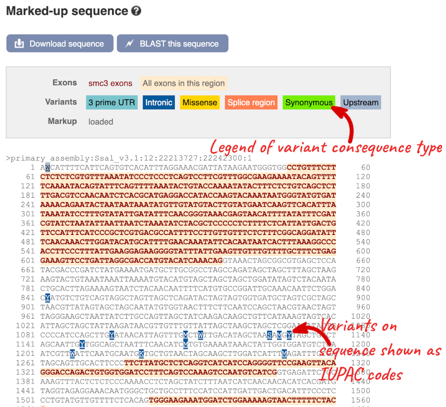
Find out more about a variant by clicking on it.
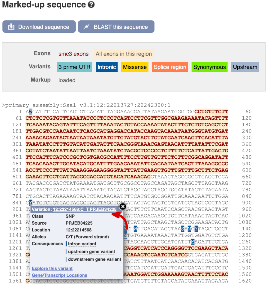
You can go to the Variation tab by clicking on the variant ID. For now, we’ll explore more ways of finding variants.
To view all the sequence variations in table form, click the Variation table link at the left of the gene tab.
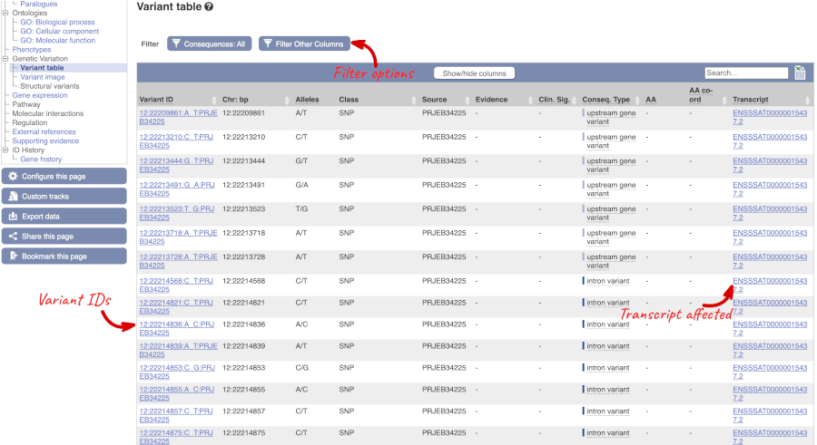
You can filter the table to only show the variants you’re interested in. For example, click on Type: All, then select the variant consequences you’re interested in.

The table contains lots of information about the variants. You can click on the IDs here to go to the Variation tab too.
Let’s have a look at variants in the Location tab. Click on the Location tab in the top bar.
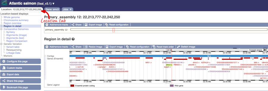
Click on Configure this page and open Variation from the left-hand menu.
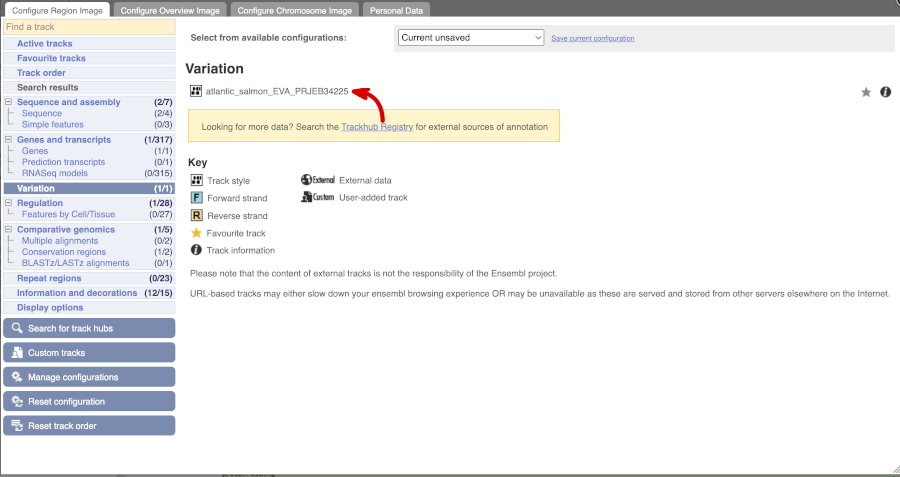
There is one track turned on by default for Atlantic_salmon_EVA_PRJEB34225
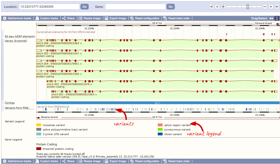
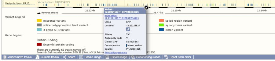
Click on a variant to find out more information. It may be easier to see the individual variants if you zoom in.
Let’s have a look at a specific variant. If we zoomed in we could see the variant 12:22221527:T_C:PRJEB34225 in this region, however it’s easier to find if we put 12:22221527:T_C:PRJEB34225 into the search box. Click through to open the Variation tab.
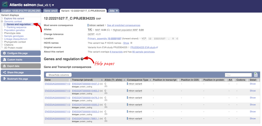
The icons show you what information is available for this variant. Click on Genes and regulation, or follow the link at the left.
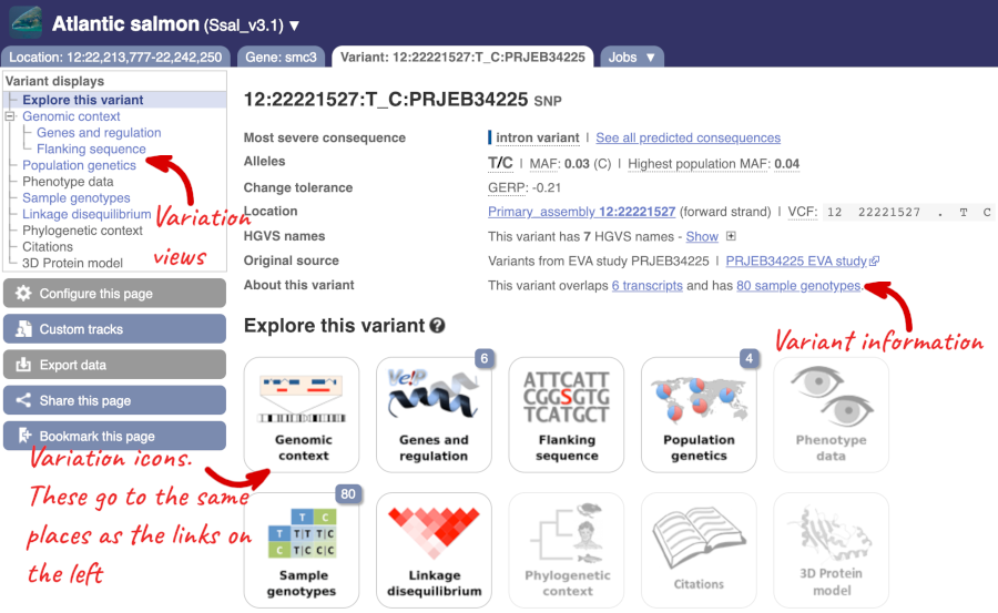
This variant is found in six transcripts of the smc3 (ENSSSAG00000007113) gene. It has not been associated with any regulatory features or motifs.
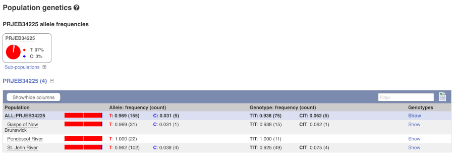
Let’s look at population genetics. Either click on Explore this variant in the left hand menu then click on the Population genetics icon, or click on Population genetics in the left-hand menu. We can see information here on Populations from the EVA study PRJEB34225.
Exploring a SNP in Atlantic salmon
The missense variant 25:3426821:C_A:PRJEB34225 is found in the Atlantic salmon hs6st2 gene.
(a) Find the page with information for 25:3426821:C_A:PRJEB34225.
(b) Is 25:3426821:C_A:PRJEB34225 a missense variation in all transcripts of the hs6st2 gene?
(c) What is the major allele in 25:3426821:C_A:PRJEB34225?
(a) Please note there is more than one way to get this answer. Either go to the Variant Table for the Atlantic salmon hs6st2 gene, and filter variants to the missense variants, or search Ensembl for 25:3426821:C_A:PRJEB34225 directly.
(b) Once you’re in the Variation tab, click on the Genes and regulation link or icon.
This SNP is found in four transcripts from two genes. It is a missense variant in hs6st2 gene and an intron variant, and downstream gene variant in ENSSSAG00000118991.
(c) Select Population genetics from the side menu.
From the Frequency data table, the PRJEB34225 allele frequencies shows that C is the major allele (95% of all population) compared to A (5% of all population).
Exploring sequence variant annotation in Atlantic salmon
(a) Find the ox2g gene for Atlantic salmon and go to the Variation table page. What is the variation name for D374H variant from EVA study PRJEB34225?
(b) Is this variant a missense variant (a Sequence Ontology term) for all transcripts that have been annotated for the ox2g gene?
(c) Why does Ensembl put the G allele first (G/C)?
(d) How many sample genotypes are available for this variant? Do all samples have the same genotype?
(a) Go to the Ensembl species page for Atlantic salmon and search for ox2g.
In the Variation Table, type e.g. 374 and/or D/H in the Filter text box.
The variation name for D374H is 21:28064636:G_C:PRJEB34225.
(b) Click on 21:28064636:G_C:PRJEB34225.
No, 21:28064636:G_C:PRJEB34225 is missense for three ox2g transcripts (ENSSSAT00000055888.2, ENSSSAT00000055982.2, ENSSSAT00000214738.1). It has the intron variant consequence for two ox2g transcripts (ENSSSAT00000195834.1 and ENSSSAT00000055943.2). Note: ox2g has five transcripts (https://feb2023.archive.ensembl.org/Salmo_salar/Gene/Variation_Gene/Table?db=core;g=ENSSSAG00000039791;r=21:27997093-28104998;source=PRJEB34225;v=21:28064636:G_C:PRJEB34225;vdb=variation;vf=21:28064636:G_C:PRJEB34225).
(c) In Ensembl, the allele that is present in the reference genome assembly is put first, i.e. G. In the literature normally the major allele (in the population of interest) is put first. In the case of 21:28064636:G_C:PRJEB34225 the allele in the reference genome is the major allele in all populations studied (Gaspe of New Brunswick, Penobscot River, St. John River).
(d) Click on Sample genotypes on the left menu.
This variant has 80 sample genotypes. It has 16 homozygous G/G genotypes in Gaspe of New Brunswick, 11 homozygous G/G in Penobscot River and in St. John River population, two of the 53 samples have heterozygous G/C genotype and the rest have homozygous G/G genotype. This information comes from EVA study PRJEB34225.
VEP
We have identified four variants in salmon:
12:22217409:G_C:PRJEB34225, 12:22215848:G_C:PRJEB34225, 12:22216033:C_G:PRJEB34225, 12:22215848:G_C:PRJEB34225
We will use the Ensembl VEP to determine:
- If the variants have been annotated in Ensembl already
- If genes are affected by the variants
Go to the front page of Ensembl and click on Variant Effect Predictor in the Tools section or click on VEP in the top header.
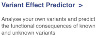
This page contains information about the VEP, including a link for downloading the script version of the tool. Click on the Launch VEP button to open the input form.
Lets input the variants data in VCF format:
Chromosome Position Name Reference Alternative
Put the following into the Input data box:
12  22217409  .  G  C
12  22215848  .  G  C
12  22216033  .  C  G
12  22215848  .  G  C
The VEP will detect automatically that the data is in VCF format.
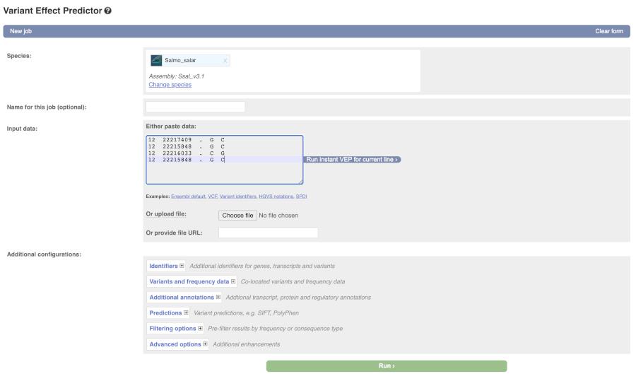
There are further options that you can choose for your output. These are categorised as Identifiers, Variants and frequency data, Additional annotation, Predictions, Filtering options and Advanced options. Let’s open all menus and take a look.
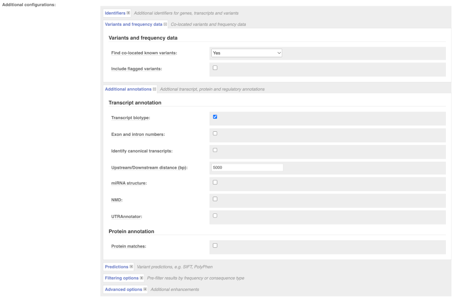
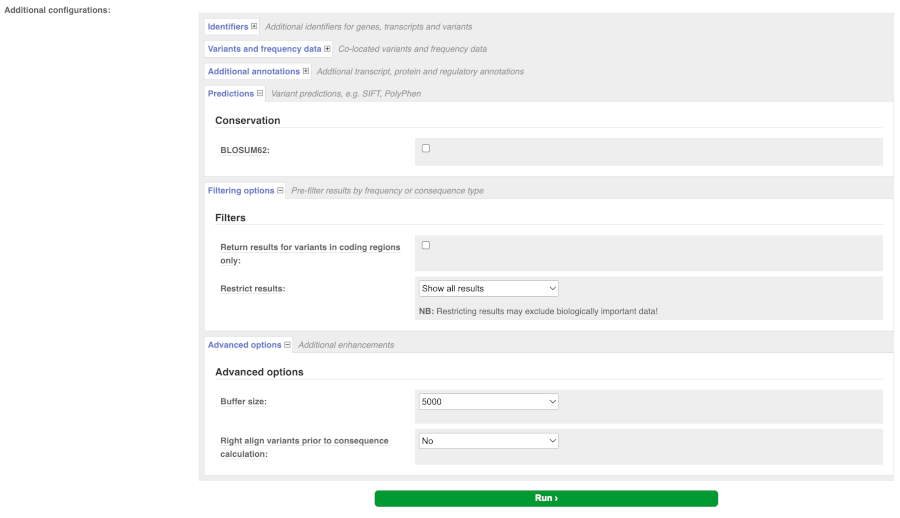
Hover over the options to see definitions.
When you have selected everything you need, scroll right to the bottom and click Run.
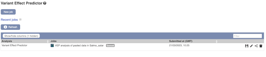
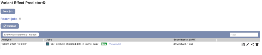
The display will show you the status of your job. It will say Queued, then automatically switch to Done when the job is done, you do not need to refresh the page. You can save, edit, share or delete your job at this time. If you have submitted multiple jobs, they will all appear here.
Click on View Results once your job is done.
In your results you will see a graphical and table summary of the data as well as a table with the detailed results.
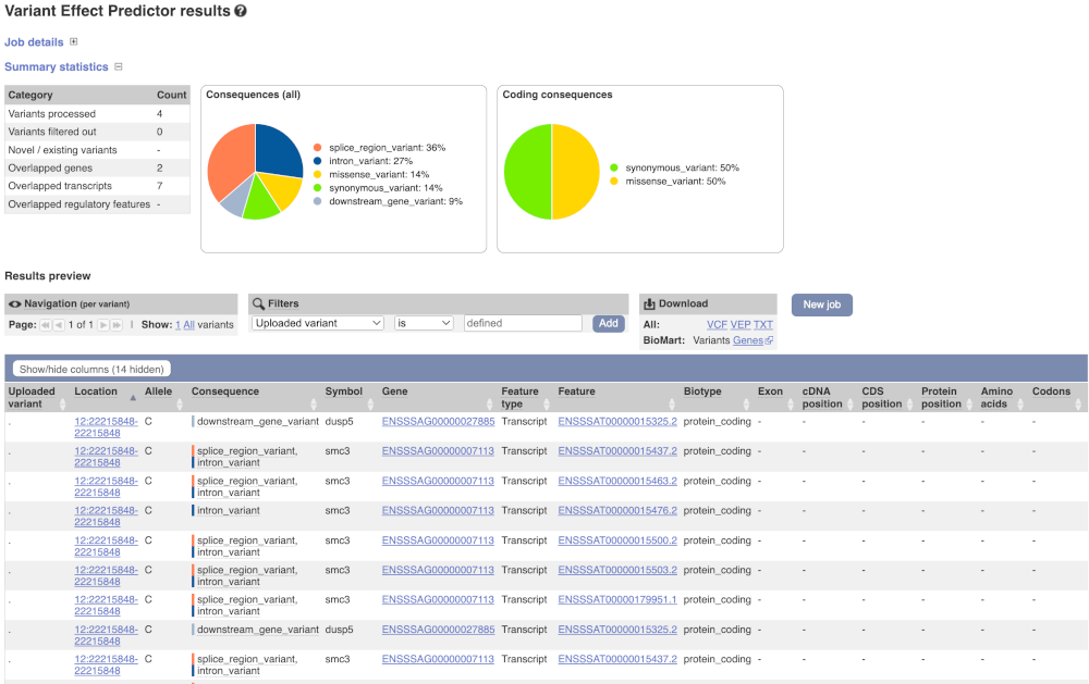
VEP cdk5r1b Atlantic salmon
We have identified a few variants in Atlantic salmon (Salmo salar):
- chr 28, genomic coordinate 1777645, alleles C/T
- chr 28, genomic coordinate 1777906, alleles G/A
- chr 28, genomic coordinate 1786995, alleles T/G
(a) Which genes and transcripts do these variants map to?
(b) Do these variants result in a change in the proteins encoded by any of the Ensembl genes? Which genes?
Go to www.ensembl.org and click on the Variant Effect Predictor link on the homepage. Click Launch VEP.
Choose Atlantic salmon as the species and copy the following into the Paste data text box:
28 1777645 1777645 C/T var1.
28 1777906 1777906 G/A var2.
28 1786995 1786995 T/G var3.
Note: Variation data input can be done in a variety of formats. See more details here http://www.ensembl.org/info/docs/variation/vep/vep_formats.html
Click Run.
When your job is listed as Done, click View Results.
You will get a table with the consequence terms from the Sequence Ontology project (http://www.sequenceontology.org/) (i.e. synonymous, missense, downstream, intronic, 5’ UTR, 3’ UTR, etc) provided by VEP for the listed SNPs. You can also upload the VEP results as a track and view them on Location pages in Ensembl.
The variants overlaps three genes (six transcripts of psmd11b, four transcripts of cdk5r1b and one transcript of ENSSSAG00000096896 gene)
Variant 28_1777906_G/A overlaps cdk5r1b gene and resulted in amino acid change at position 109 and 116 (Ser to Leu), variant 28_1777645_C/T also overlaps cdk5r1b gene and resulted in amino acid change at position 96 and 203 (Arg to His).
VEP analysis of variant in Atlantic salmon
You have performed sequencing and variant-calling experiments for Atlantic salmon. You have a few variants in the VCF format from this experiment:
25 4297825 . G A.
25 4293985 . C G.
25 4294047 . G T.
25 4294047 . G T.
25 4270019 . G A.
(a) How many variants were analysed? How many are novel?
(b) How many genes and transcripts are affected by these variants?
(c) Do any of the variants have different consequences for different transcripts?
(d) Can you export all the results to a VCF file?
Go to www.ensembl.org and click on the Variant Effect Predictor link on the homepage. Click Launch VEP.
Choose Atlantic salmon as the species and enter the five variants from the exercise.
Note: Variation data input can be done in a variety of formats. See more details here http://www.ensembl.org/info/docs/variation/vep/vep_formats.html
Click Run.
When your job is listed as Done, click View Results.
(a) Five variants were analysed, none of these variants are novel.
(b) Only one gene (cdc16) is affected by these variants. It has ten transcripts, all of which are affected.
(c) Yes. These variants have the missense_variant, intron_variant and downstream_gene_variant consequences for the different transcripts of cdc16 gene.
(d) At the top right of the table there is an option to download data. Click on VCF for the All option. Open the VCF file you have downloaded in a text editor. You can see that VEP adds annotation in the INFO column of the VCF file.
Comparative genomics
Demo: gene trees and homology predictions
Comparative Genomics
Gene trees
Let’s look at the homologues of the Salmo salar (Atlantic salmon) gh1 (ENSSSAG00000055013) gene. This gene codes for growth hormone 1. Search for the gene and go to the Gene tab.
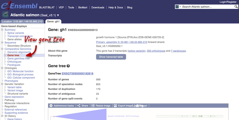
Click on Comparative Genomics: Gene tree. This will display the current gene in the context of a phylogenetic tree used to determine orthologues and paralogues.
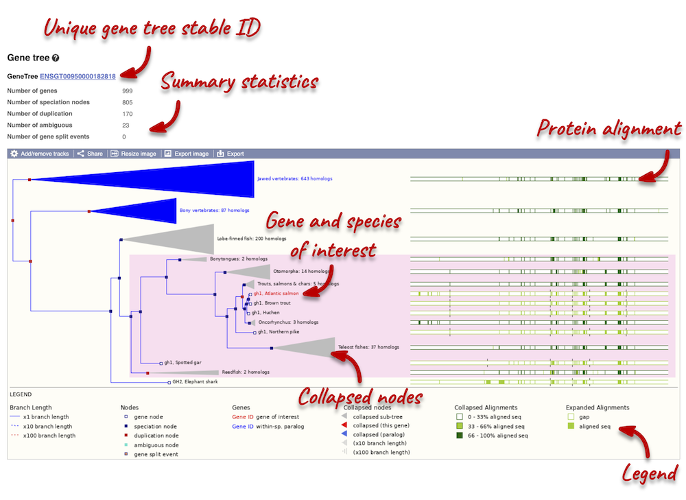
The phylogeny is displayed on the left-hand side. Protein alignments are displayed on the right-hand side. You can find a legend at the bottom of the view.
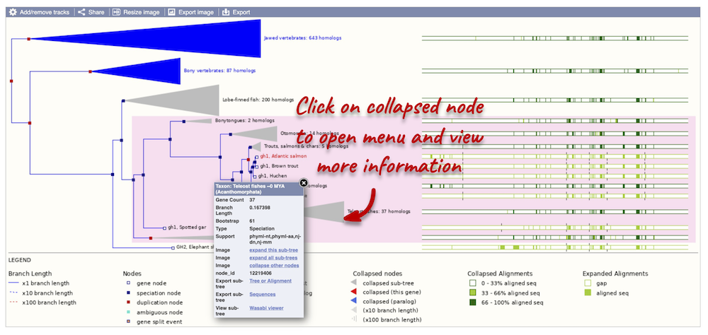
Funnels within the phylogeny indicate collapsed nodes. Click on a node (coloured triangle) to open a menu. We can then see what type of node this is, some statistics and options to expand or export the sub-tree.
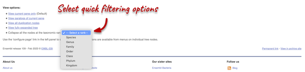
There are some quick filtering options below the image, where you can add paralogues, and quickly expand or collapse nodes.
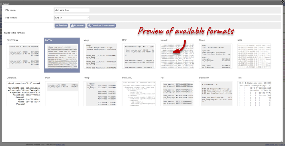
You can download the tree in a variety of formats. From the pop-up above, you can click to export the sub-tree (everything to the right of the node). Alternatively, click on the Export icon ![]() in the bar at the top of the image to get a pop-up where you can choose your format. You can preview this file before you download.
in the bar at the top of the image to get a pop-up where you can choose your format. You can preview this file before you download.
Homologues
We can look at homologues in the Orthologues and Paralogues pages, which can be accessed from the left-hand menu. If there are no orthologues or paralogues, then the name will be greyed out. Click on Comparative Genomics: Orthologues to see the orthologues available. In the first table, you will find a summary of orthologues by species sets. Let’s select the Fish set only. There are 64 species in this set.
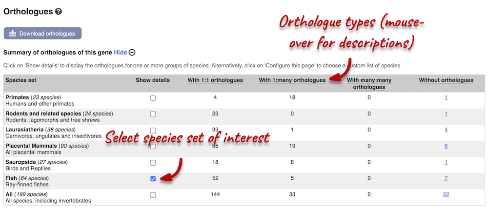
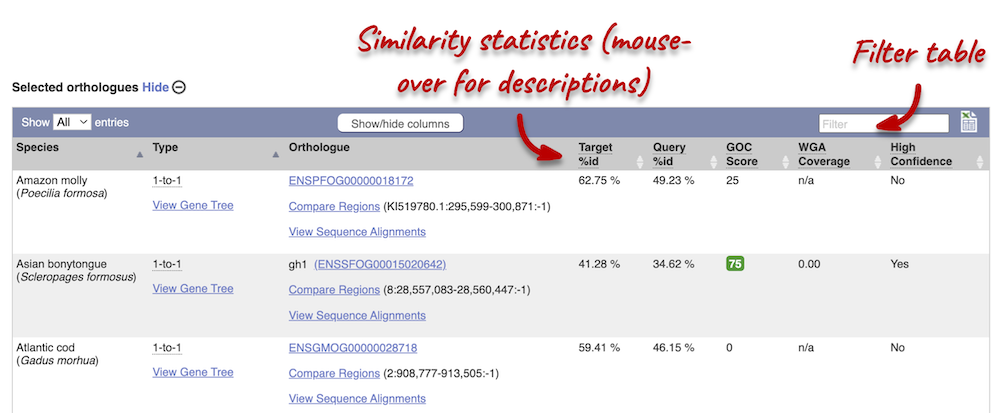
In the second table, you will find orthologue details per species:
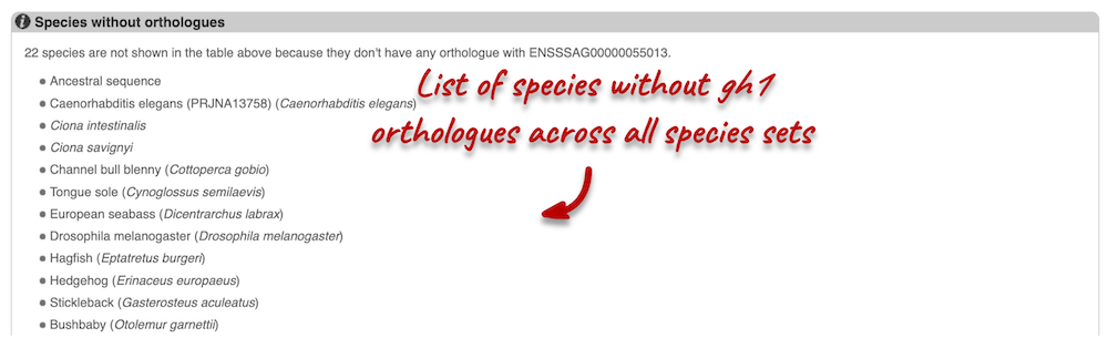
Scroll to the bottom of the page to see a list of the species that do not have any orthologues with gh1 in Atlantic salmon… there are a lot!
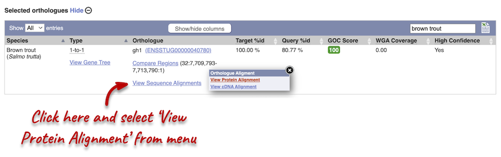
Let’s compare the Atlantic salmon and Salmo trutta (brown trout) homologues. Search for brown trout in the Orthologues table above using the filter at the top right-hand corner. Links from the orthologue allow you to view the two orthologues within a gene tree, see the gene entry for brown trout, compare the regions of the orthologues, or view protein and cDNA alignments. Click on View Sequence Alignments, and then View Protein Alignment for the brown trout orthologue.
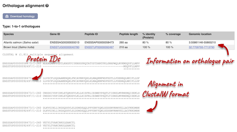
The protein alignment is displayed in ClustalW format. If you are unfamiliar with this format, you can find information in the Ensembl help pages. You can also export the alignment in other formats by clicking the Download homology button at the top of the alignment.
Demo: Whole-genome alignments
Alignments in the Region in Detail view
Pairwise alignments
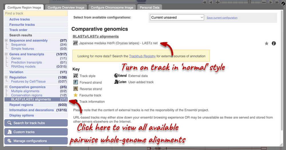
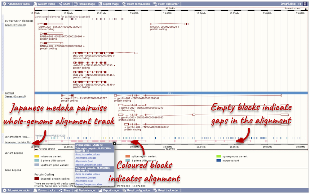
Let’s look at some of the comparative genomics views in the Location tab. Go to the region 21:19789800-19872000 in Salmo salar (Atlantic salmon). This region contains a number of different genes. We want to find out if there are any specific regions that align with the Oryzias latipes (Japanese medaka). To do this, we need to look at a LASTz pairwise alignment between the Atlantic salmon and Japanese medaka species. We can look at individual species comparative genomics tracks in the Region in detail view by clicking on Configure this page. In the Comparative genomics section, go to BLASTz/LASTz alignments and turn on the Japanese medaka track in the normal format. Save and close the menu.
We now have a new track, which shows aligned regions in pink blocks. Gaps in the alignment are displayed as empty blocks. Alignments to a single chromosome are presented in a single row. You will find multiple rows of alignments will be shown if the region aligns to more than one chromosome. Click on an aligned region. From the pop-up menu we can see that region of interest only aligns to chromosome 21 in Japanese medaka, and therefore only one row of alignment is shown in the display
Highly conserved region across the 65 fish EPO-Extendes set align with the
Multiple alignments
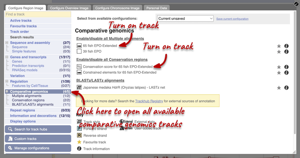
Atlantic salmon is part of the 39 fish EPO and 65 fish EPO-Extended comparative genomics analyses. You can view multiple whole-genome alignments on the Region in detail view. Configure this page, go to Comparative genomics: Multiple alignments and turn on the 65 fish EPO-Extended track. Also turn on the Conservation score for 65 fish EPO-Extended and Constrained elements for 65 fish EPO-Extended under Comparative genomics: Conservation regions. You can read more about GERP scores in the Ensembl Comparative Genomics documentation pages. This will show us if any regions are highly conserved within the species set. Save and close the menu.
Any conserved regions are shown in the 65 way GERP elemenst track. You can find corresponding conservation scores in the 65 way GERP scores track underneath. These tracks indicate regions of high conservation between species, considered to be “constrained” by evolution.
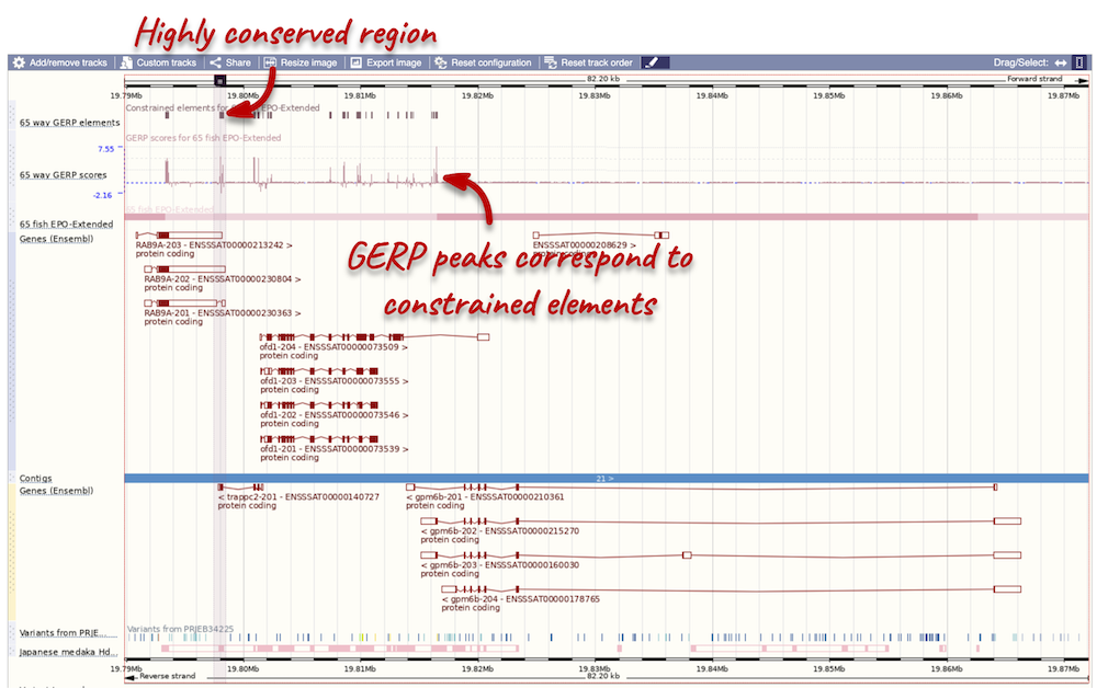
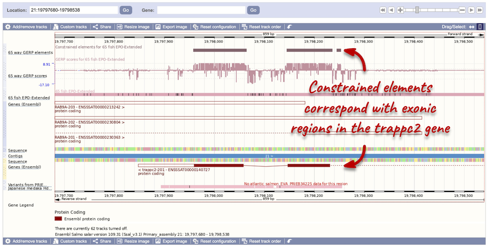
You can zoom into a highly conserved region by dragging your mouse across the region you want to zoom into, and selecting Jump to region in the pop-up menu. Zoomed in, you will be able to see that the constrained elements actually correspond to exonic regions of the trappc2-201 transcript.
Pairwise sequence alignments
We can look at the nucleotide sequence alignment between Atlantic salmon and Japanese medaka. Click on Comparative Genomics: Alignments (text) in the left-hand menu.
Click on Select an alignment. Under Pairwise, select Japanese medaka and click Apply at the bottom of the menu to save and close. 5 alignment blocks of different lengths are available.
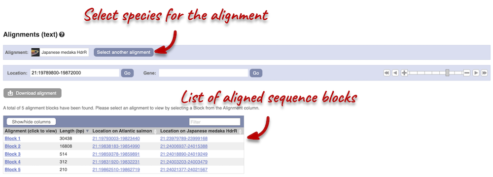
Click on Block 1. You will see a list of aligned regions in Atlantic salmon and Japanese medaka. Scrolling down you will find the nucleotide sequence alignment of the two species. Exons are shown in red.
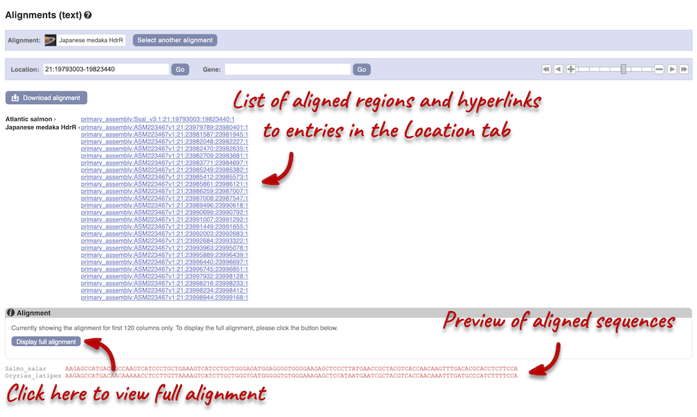
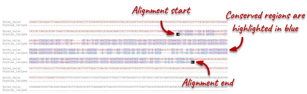
Configure this page on the left. In the pop-up menu, you can turn on the options to view Show conservation regions and Mark alignment start/end. This will add highlights where the sequence matches. Save and close the menu and click on Display full alignment.
Region comparison
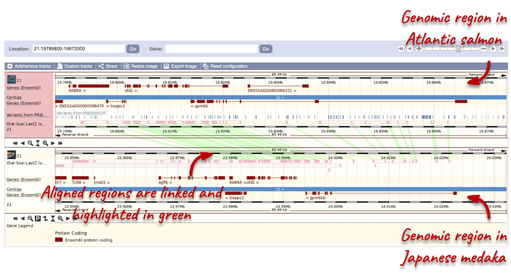
To compare the two genomic regions visually, go to Comparative Genomics: Region Comparison in the left-hand panel. To add species to this view, click on the Select species or regions button. Select Japanese medaka again then close the menu. This page, similar to the Region in detail view, shows the chromosome positions (for both species) first. We can see the location of this alignment on chromosome 21 in Japanese medaka. You can scroll down to the Region in detail display. Here, you can view the aligned regions (highlighted in green) between the two species.
You can add the same tracks as those in the Region in detail view to this region comparison. Click on Configure this page to open the menu and select your tracks of interest.
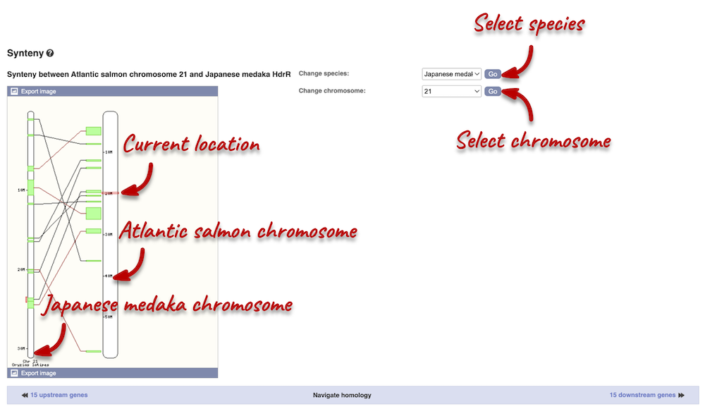
Synteny
We can view large-scale syntenic regions for our chromosome of interest. Click on Comparative Genomics: Synteny in the left-hand panel. Select Japanese medaka from the Species drop-down on the right-hand side. Black linking lines indicate sequences are oriented in the same direction, red linking lines indicate the sequences are inverted.
Exploring European seabass pax6b orthologues
Go to Ensembl to answer the following questions:
-
How many orthologues are predicted for the Dicentrarchus labrax (European seabass) pax6b gene across ray-finned fishes?
-
How much sequence identity does the Sparus aurata (Gilthead seabream) protein have to the European seabass one?
-
Can you tell which end of the pax6b protein is more conserved between these two species by looking at the orthologue alignment?
- From the Ensembl homepage, choose European seabass from the drop-down list and search for
pax6b. Click through to the Gene tab view. Click on Comparative Genomics: Orthologues at the left side of the page to see all the orthologous genes.From the summary table, we can see that the European seabass has 52 1-to-1 orthologues and 9 1-to-many orthologues in the ray-finned fishes species list.
- Search for
Gilthead seabreamin the orthologues table below.The percentage of identical amino acids in the Gilthead seabream protein (the orthologue) compared with the gene of interest, i.e. the European seabass pax6b (the target species/gene), is 99.78%. This is known as the Target%id.
The identity of the gene of interest (European seabass pax6b) when compared with the orthologue (Gilthead seabream pax6b, the query species/gene) is 99.78% (the Query %id).
Note that any difference in the values of the Target and Query %id reflects the different protein lengths for the two orthologues. In the case of the European seabass and Gilthead seabream, the identity is the same as both proteins are 457 amino acids long.
- Click on the View Sequence Alignments link in the Orthologue column to View Protein Alignment in ClustalW format.
Conserved amino acids are indicated by asteriks (*). You can find more information about the ClustalW format in our help pages. There is no difference between the N-terminus and C-terminus. The sequence is conserved around both termini.
Gene tree of the turbot clocka gene
Let’s look at the gene tree of clocka in Scophthalmus maximus (turbot). This gene codes for a circadian clock regulator. Use Ensembl to find the following information:
-
What is the gene tree ID for the the clocka gene in turbot? How many genes are in this tree? How many genes are in the super-tree?
-
According to the gene tree, which species matches the European seabass sequence the most? What is the gene ID for this homologue?
-
Export the gene tree as an image and in Newick format.
- Search for clocka in turbot. Open the Gene tab and click on Comparative Genomics: Gene tree in the left-hand panel.
The gene tree ID is ENSGT00940000157580. There are 264 genes in this tree. There are a total of 1,447 genes in the super-tree.
- Find the turbot clocka node in the gene tree (this is highlighted in red font). Look for the most closely-related gene by following the phylogeny.
From the phylogeny, we can see that Lates calcarifer (Barramundi perch) has the most similar sequence to the European seabass as it is the most closely-related sequence in the phylogeny.
- You can find download options at the top of the phylogeny. Click on Export image to download the image. You select which format you want to download the image as.
Click on Export to download the gene tree in different tree formats. Select Newick from the drop-down menu or the file format previews. You can also export alignments from this menu.
BioMart
Demo: BioMart
You have 4 Salmo salar (Atlantic salmon) genes:
slc45a2, igf1, sod1, ube2f
Follow these instructions to guide you through BioMart to answer the following questions:
- What are the NCBI Gene IDs for these genes?
- Are there associated functions from the Gene Ontology (GO) project that might help describe their function?
- What are the coordinates of the genes?
- What are their cDNA sequences?
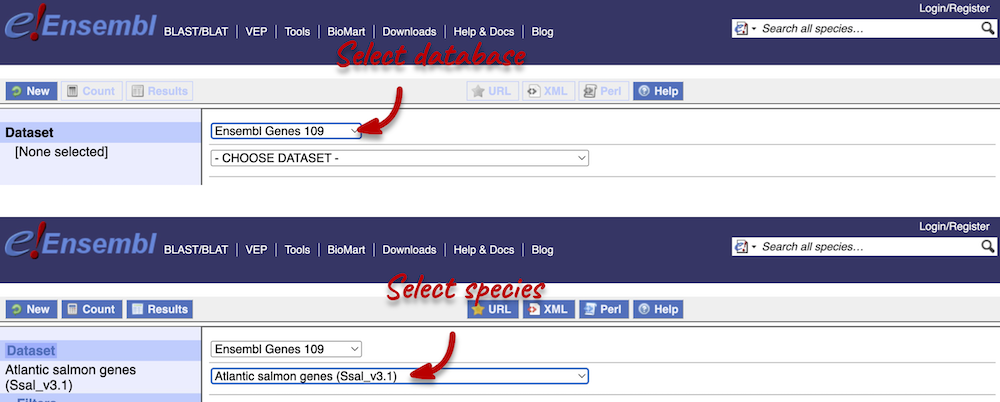
Step 1: Choose database and dataset
Click on BioMart located on the navigation bar at the top of any Ensembl page. Select Database: Ensembl Fungi Genes and Dataset: Atlantic salmon genes.
Step 2: Choose appropriate filters
We want to find these 4 genes in Atlantic salmon:
slc45a2, igf1, sod1, ube2f
We need to filter the dataset to look only at these genes. Click on Filter on the left-hand panel and open the GENES tab on the right.
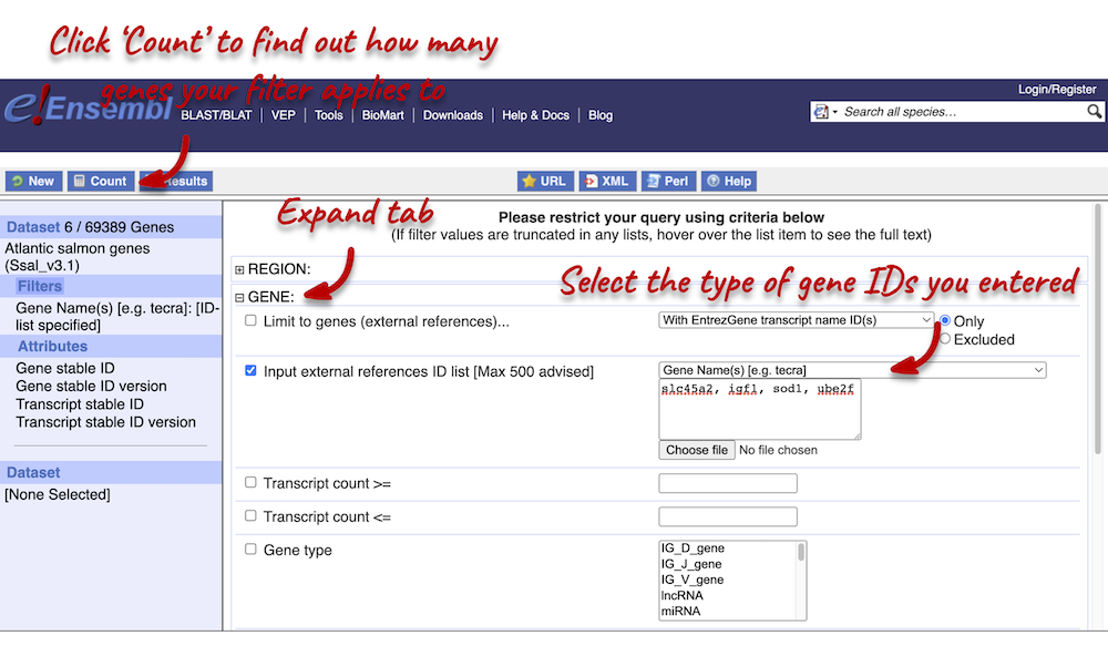
Using the count function we can see that our filter applies to 6 out of 69,389 genes in Atlantic salmon. The count is 6 (rather than 4) because gene names can be ambiguous. This means that a gene name can be given to multiple different genes.
Step 3.1: Select attributes (features)
Attributes are defined by what we would like to learn about the data. We want to find out more information about the genes’:
- NCBI IDs
- Associated GO terms
- Coordinates
- cDNA sequences
You can only select one attribute category at a time. We can answer points 1 and 3 in a single query, but we will need to do a second query to answer point 4. Make sure that Features category is selected at the top of the page. Expand the GENE tab and select the following features:
- Gene name
- Gene start
- Gene end
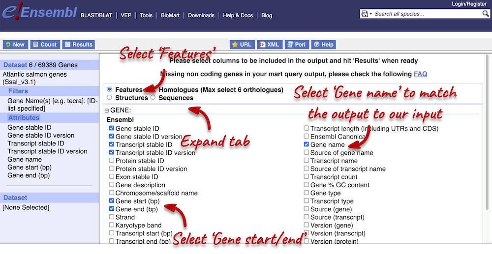
We have added the Gene name attribute, because we want to be able to match out output with our input. As we searched for gene names, we want to be able to see which features match to our given gene.
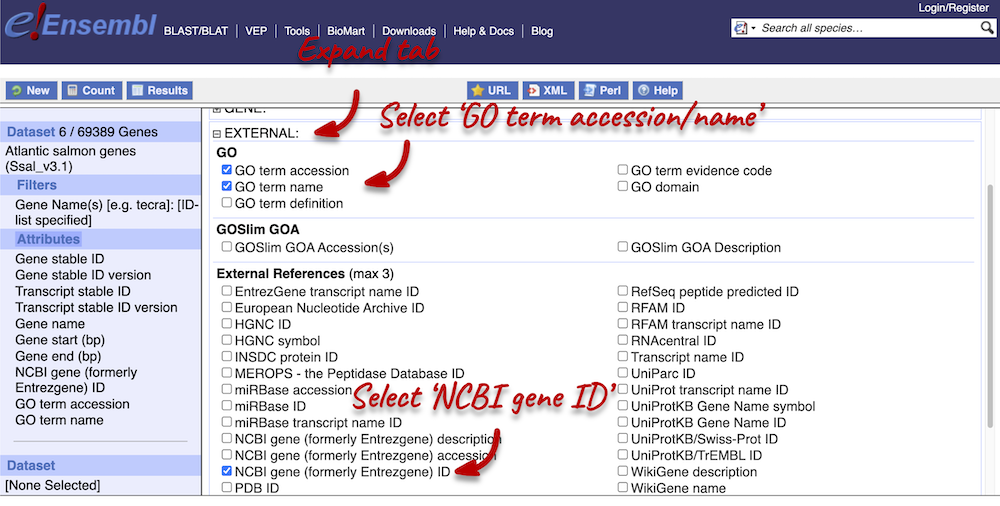
Next, expand the EXTERNAL tab. This section contains lots of identifiers from databases outside of Ensembl. Select the following features:
- NCBI IDs
- GO term accession
- GO term name
Step 4.1: Get the results (features)
You can download the data by selecting a format type (HTML, TSV, CSV or XLS) from the drop-down under Export all results to and clicking Go. The table presented shows a sub-sample of 10 results to enable you to check you have the correct attributes.
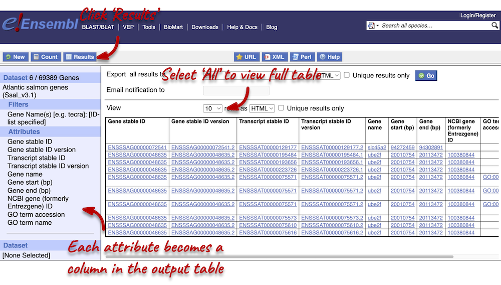
Select All rows from the drop-down menu under View to open all results in a new tab. You will notice that there are multiple results for gene names slc45a2 and ube2f. This is because the names can be ambiguous. If you focus on the Gene stable ID column, you will notice that gene names slc45a2 and ube2f will each have 2 different gene stable IDs assigned to them. Gene stable IDs are unique.
You may see multiple entries for each gene stable ID. This is because a gene can be transcribed into a number of transcripts, so you will have results for each of the transcripts (see the Transcript stable ID column). Finally, you may also notice that there are multiple entries for each transcript. This is because multiple GO terms can be associated to a single transcript (see the GO term accession column).
Step 3.2: Select attributes (sequences)
To complete the third part of the demo, we need to export the cDNA sequences of our three genes. To do this, go back to the Attributes section in the left-hand panel and select Sequences from the attributes categories at the top of the page. Expand the SEQUENCES tab and select cDNA.
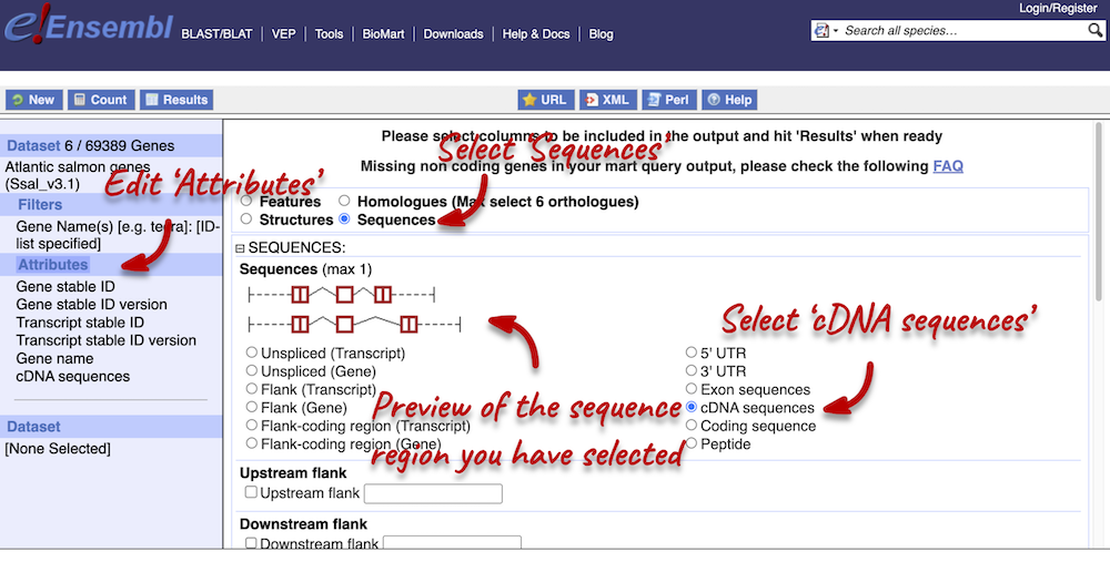
Next, expand the HEADER INFORMATION tab and select Gene name, so that we can match our output to our input again. Click Results in the left-hand panel to see your sequences.
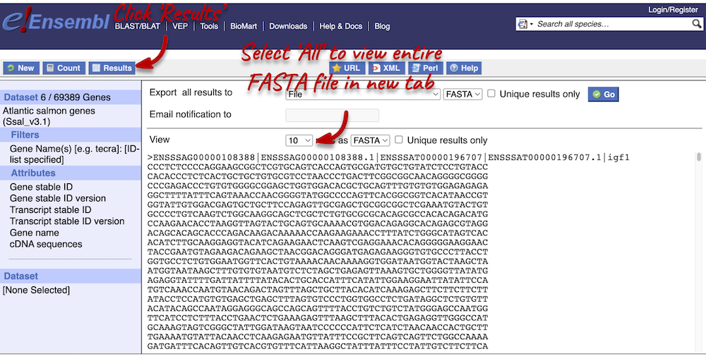
Step 4.2: Get the results (sequences)
Click on Results again in the top left-hand corner to view your cDNA sequences in FASTA format. You can find your gene and transcript stable IDs, as well as the gene name in your FASTA header, which is followed by the cDNA sequence itself.
For more details on BioMart, have a look at this publication:
Kinsella RJ, Kähäri A, Haider S, et al. Ensembl BioMarts: a hub for data retrieval across taxonomic space. Database: the Journal of Biological Databases and Curation. 2011 ;2011:bar030. DOI: 10.1093/database/bar030. PMID: 21785142; PMCID: PMC3170168.
Convert IDs using BioMart
BioMart is a very handy tool when you want to convert IDs from different databases. The following is a list of 30 gene IDs from the UniProtKB database:
Q4QY71,P52727,P40148,P29971,O42457,B9TQX2,A7YD35,A0A023I9E0,A0A0B4KJH3,A0A0B4KJK0,
A0A0B4KJW0,A0A0E3EKP4,A0A0F6MWY9,A0A0F6MX02,A0A0F6MX04,A0A0F6MX09,A0A0F6MX23,A0A0F6MX34,A0A0F6MX41,A0A0F6MX46,
A0A0F6MX65,A0A0F6MX78,A0A1D6X7G2,A0A2D1CGZ1,A0A2D1CGZ5,A0A2D1CH18,A0A2R2YUP1,S4SIT9,X2CQB0,A0A0F6MX77
Use BioMart in Ensembl to generate a list that shows to which Ensembl gene stable IDs and to which gene names these UniProtKB gene name IDs correspond. How many different transcripts do the 30 genes correspond to? Why do multiple transcripts correspond to a single UniProtKB gene ID?
-
Go to BioMart. You can find a shortcut to the tool on any Ensembl page in the navigation bar at the top of the page. Click New in the top left-hand menu if you need to start a new query. Select the Ensembl Genes database. Choose the Gilthead seabream genes dataset.
-
Click on Filters in the left panel. Expand the GENE section. Select Input external references ID list). Enter the list of IDs in the text box. Don’t forget to select the correct ID format from the drop-down menu. Select UniProtKB Gene Name ID (HINT: you may have to scroll down the drop-down menu to find this). Count the number of genes your filter applies to. This should be 30 / 27,714.
-
Click on Attributes in the left panel. Select the Features attributes page. Expand the GENE section. Here, the Gene stable ID and Transcript stable ID are already selected by default. Keep those selection and also add Gene name. Next, expand the EXTERNAL section and select UniProtKB Gene Name ID. We are adding this to be able to match our output to our input.
-
Click the Results button on the toolbar. Select View: All rows as HTML to view your results in a new tab, or export all results to a file directly to your local machine. You can open the table in Excel and count the number of unique transcript IDs in the Transcript stable ID column.
There are 46 unique transcript IDs.
Multiple transcripts can correspond to a single UniProtKB gene ID because a gene is made up of a set of transcripts: multiple transcripts can be transcribed from a single gene.
Exporting homologues with BioMart
Go to Ensembl’s BioMart. For a list of Cyprinus carpio carpio (common carp) Ensembl genes, export the Oncorhynchus mykiss (rainbow trout) orthologues and their coordinates:
ENSCCRG00000054216,ENSCCRG00000032455,ENSCCRG00000022461,ENSCCRG00000066160,ENSCCRG00000028244,
ENSCCRG00000006279,ENSCCRG00000072009,ENSCCRG00000031644,ENSCCRG00000044263,ENSCCRG00000075394
Do all of these genes have a homologue in rainbow trout?
-
Go to BioMart (you can find a shortcut in the navigation bar at the top of any Ensembl page) and click New. Choose the Ensembl Genes database. Choose the Common carp genes dataset.
-
Click on Filters in the left panel. Expand the GENE. Enter the gene list in the Input external references ID list box. Gene stable ID(s) should already be selected by default.
- Click on Attributes in the left panel. Select the Homologues attributes at the top of the page. Expand the GENE section. Deselect Gene stable ID version, Transcript stable ID and Transcript stable ID version. Expand the ORTHOLOGUES [P-T] section. Select the following attributes under Rainbow trout Orthologues:
- Rainbow trout gene stable ID
- Rainbow trout gene name
- Rainbow trout chromosome/scaffold start (bp)
- Rainbow trout chromosome/scaffold end (bp)
- Click Results. Select View: All rows as HTML.
All but ENSCCRG00000022461 and ENSCCRG00000075394 have a homologue in rainbow trout. Your output should also included the gene ID and name in rainbow trout and their coordinates.